


Figure
1.
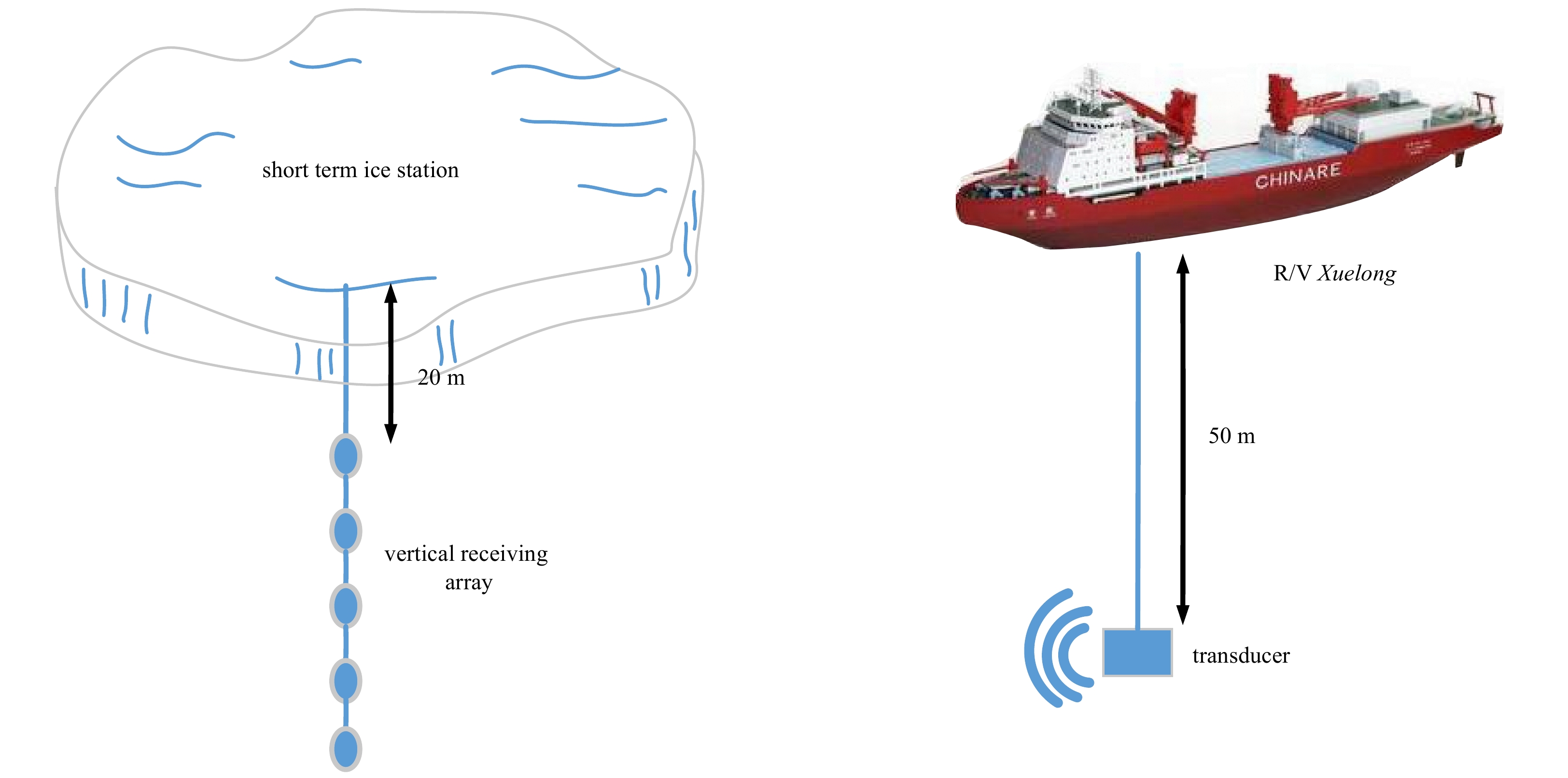
The schematic diagram of underwater acoustic communication experiment.
| Citation: | Yanan Tian, Xiao Han, Jingwei Yin, Hongxia Chen, Qingyu Liu. An improved least mean square/fourth direct adaptive equalizer for under-water acoustic communications in the Arctic[J]. Acta Oceanologica Sinica, 2020, 39(9): 133-139. doi: 10.1007/s13131-020-1653-6

|
With the rapid development of various applications in the Arctic in recent years, more and more ocean observation equipment such as underwater unmanned vehicle (UUV) is being used in the Arctic to gain insight into the temporal and spatial processes below the ice surface (Wang et al., 2017; Li et al., 2019). However, the thick ice covered in the Arctic prevents underwater platforms from communicating with the satellites, which makes acoustics the only means of data transmissions under ice surface. Different from open-water environment, under-ice environment can introduce some new problems for acoustic communication such as larger transmission loss, severe Doppler effect, and impulsive noise. The key feature of the typical Arctic sound speed profile is that the minimum sound speed resides at the ice-water interface (Freitag et al., 2012). According to the ray theory, all of the acoustic energy in this typical Arctic environment will interact with the ice cover. Because of the roughness of the ice cover, acoustic interactions with the ice cause significant scattering and therefore significant losses. When communicating in the floating ice area, the acoustic rays which are reflected by time-varying rough ice surface can introduce random Doppler effect which makes it difficult to compensate the phase of received signals. There are also many ice cracking or ice collision activities in the Arctic, producing a lot of impulsive noise which makes it challenge work to achieve robust communication performance.
The inter-symbol interference (ISI) caused by multipath spread and the Doppler shift owing to the relative motion make the channel equalization at the receiving end a challenging task for underwater acoustic (UWA) communications (Berger et al., 2010; Liu et al., 2017). Two representative methods in channel equalization are frequency domain equalization (Falconer et al., 2002) and time domain equalization (Vanbleu et al., 2006). The former has a lower computational complexity, but it cannot track channel changes in time for the reason that it operates in block units. Two important classifications in time domain equalization are direct adaptive equalizer (DAE) which obtains the equalizer coefficients directly from the received data, and channel estimation based equalizer (CEBE) using the received signal to get the channel taps and then calculating the equalizer coefficients (Pelekanakis and Chitre, 2013). When the signal to noise ratio (SNR) is low, the performance of the two is similar, but the calculation complexity of DAE is low (Lee and Cox, 1997). The DAE with an embedded phase-locked loop (PLL) has been successfully applied in UWA channel equalization for many years (Stojanovic et al., 1993).
The UWA equalizer exhibits sparse features due to the sparsity of the UWA channel itself, which means that most coefficients are close to zero (Vlachos et al., 2012; Li and Preisig, 2007). Inspired by sparse adaptive filtering theory, attempts at combining sparse nature with adaptive equalizers have gained considerable interest. Pelekanakis and Chitre (2010) apply improved proportionate normalized least mean square (IPNLMS) to the decision feedback equalization (DFE). The results prove its superiority when sparse channel is encountered and it also shows robustness for non-sparse channel. Duan et al. (2018) use the IPNLMS to update the coefficients of the Turbo equalizer. It speeds up the convergence of large taps with good tracking ability and low computational complexity. Chen et al. (2009) add the norm penalties to the cost function and exploit them as sparse regularizations, thus obtaining zero-attracting LMS (ZA-LMS) and reweighted ZA-LMS (RZA-LMS), which gain additional performance. In Tao et al. (2017), authors propose selective ZA-NLMS (SZA-NLMS) equalization method. Compared with ZA-NLMS, it does not impose the same penalty on all coefficients uniformly, but limits the scope of constraints, further improving the performance of the equalizer. The LMS equalizer is widely used due to the simplicity of operation and small amount of calculation. However, it is sensitive to input signals and SNR, and the performance is severely degraded especially under low SNR (Guan et al., 2013b). Recursive least square (RLS) can overcome such problems, and methods employing RLS constrained by sparse features have also appeared. RLS penalized by a general convex function is proposed in (Eksioglu and Tanc, 2011). It can adaptively adjust the strength of the sparse constraint according to certain criteria, so the performance improves significantly. However, the computational complexity of RLS increases as the square of the length of the equalizer (Eksioglu, 2014). When the UWA channel multipath expansion is severe, the computational complexity is extremely high. The least mean fourth (LMF) based on high order moment is also an effective method to overcome noise (Walach and Widrow, 1984). It utilizes the fourth power instead of the square power of the equalization error. According to the theory in Mendel (1991), the high-order energy filter can suppress the noise interference better, and can overcome the shortcomings of the LMS. However, its computational complexity is still very high. Combining the advantages of LMS and LMF, the LMS/F algorithm can effectively improve the performance of LMS without sacrificing its simplicity and stability. The performance of LMS/F has proven to be better than that of traditional LMS and LMF (Guan et al., 2013b). Using the sparse nature of the channel, the ZA-LMS/F and RZA-LMS/F channel estimation algorithms constrained by the
The rest of the paper is organized as follows: Section 2 specifically gives the derivation process of adaptive norm LMS/F-DAE (AN-LMS/F-DAE); in Section 3, we process the experimental data from the 9th Chinese National Arctic Research Expedition to verify its reliability and effectiveness; Section 4 summarizes the whole paper.
Note: the vector is shown in bold black. The superscripts “
The output of a DAE at instant n is
| $$ {J_n} \!=\! e_n^2 \!-\! \varepsilon \ln (e_n^2 \!+\! \varepsilon) \!+\! {\gamma _w}||{{{w}}_n}||_p^p \!+\! {\gamma _f}||{{{f}}_n}||_p^p. $$ | (1) |
The first two terms in Eq. (1) are the same as those in standard LMS/F, where
| $$ \left\{\begin{split} & {{{{w}}_{n + 1}} \!\!= {{{w}}_n} \!-\! {\mu _w}\frac{{\partial {J_n}}}{{\partial {{w}}_n^*}}}\\ & {{{{f}}_{n + 1}} \!=\! {{{f}}_n} \!-\! {\mu _f}\frac{{\partial {J_n}}}{{\partial {{f}}_n^*}}} \end{split}\right. , $$ | (2) |
where
| $$ \begin{split} \frac{{\partial {J_n}}}{{\partial {{w}}_n^*}} =& \frac{{\partial (e_n^2 - \varepsilon \ln (e_n^2 + \varepsilon))}}{{\partial {{w}}_n^*}} + {\gamma _w}\frac{{\partial ||{{{w}}_n}||_p^p}}{{\partial {{w}}_n^*}}\\ = &e_n^{\rm{*}}\frac{{\partial {e_n}}}{{\partial {{w}}_n^*}} - \varepsilon \frac{{e_n^{\rm{*}}}}{{e_n^2 + \varepsilon }}\frac{{\partial {e_n}}}{{\partial {{w}}_n^*}} + {\gamma _w}\frac{p}{2}{{({{{w}}_n}{{w}}_n^*)}^{\frac{p}{2} - 1}}{{{w}}_n}\\ = &(e_n^{\rm{*}} - \varepsilon \frac{{e_n^{\rm{*}}}}{{e_n^2 + \varepsilon }})\frac{{\partial {e_n}}}{{\partial {{w}}_n^*}} + \frac{{{\gamma _w}p}}{2}\frac{{{{{w}}_n}}}{{|{{{w}}_n}{|^{2 - p}}}}\\ = & {- \frac{{e_n^{\rm{*}}e_n^2}}{{e_n^2 + \varepsilon }}{e^{ - j\theta }}{{{r}}_n} + \frac{{{\gamma _w}p}}{2}\frac{{{{{w}}_n}}}{{|{{{w}}_n}{|^{2 - p}}}}}. \end{split} $$ | (3) |
Note that
| $$ \begin{split} \frac{{\partial {J_n}}}{{\partial {{f}}_n^*}} &= \frac{{\partial (e_n^2 - \varepsilon \ln (e_n^2 + \varepsilon))}}{{\partial {{f}}_n^*}} + {\gamma _f}\frac{{\partial ||{{{f}}_n}||_p^p}}{{\partial {{f}}_n^*}}\\ & ={ \frac{{e_n^{\rm{*}}e_n^2}}{{e_n^2 + \varepsilon }}{{{\tilde{ x}}}_n} + \frac{{{\gamma _f}p}}{2}\frac{{{{{f}}_n}}}{{|{{{f}}_n}{|^{2 - p}}}}} . \end{split}$$ | (4) |
Bring Eqs (3) and (4) into Eq. (2) to get the update equation as:
| $$ {{{w}}_{n + 1}} = {{{w}}_n} + {\mu _w}\frac{{e_n^{\rm{*}}e_n^2}}{{e_n^2 + \varepsilon }}{{\rm{e}}^{ - j\theta }}{{{r}}_n} - \frac{{{\mu _w}{\gamma _w}p}}{2}\frac{{{{{w}}_n}}}{{|{{{w}}_n}{|^{2 - p}}}}, $$ | (5) |
| $$ {{{f}}_{n + 1}} = {{{f}}_n} - {\mu _f}\frac{{e_n^{\rm{*}}e_n^2}}{{e_n^2 + \varepsilon }}{{\tilde{ x}}_n} - \frac{{{\mu _f}{\gamma _f}p}}{2}\frac{{{{{f}}_n}}}{{|{{{f}}_n}{|^{2 - p}}}}. $$ | (6) |
The first two terms of Eqs (5) and (6) are the LMS/F update formulas when no sparse constraints are applied. It can be seen that when
| $$ \left\{\begin{split} &{{{w}}_{n + 1}} = {{{w}}_n} + {\mu _w}\frac{{e_n^{\rm{*}}e_n^2}}{{e_n^2 + \varepsilon }}{{\rm{e}}^{ - j\theta }}{{{r}}_n} - \frac{{{\mu _w}{\gamma _w}{{{p}}_w}}}{2}\frac{{{{{w}}_n}}}{{|{{{w}}_n}{|^{2 - {{{p}}_w}}}}}\\ & {{{p}}_w} = [{p_{w,0}}\;{p_{w,1}}\;{p_{w,2}} \cdots {p_{w,K}}] \end{split}\right. , $$ | (7) |
| $$ \left\{\begin{split} &\,{{{f}}_{n + 1}} = {{{f}}_n} - {\mu _f}\frac{{e_n^{\rm{*}}e_n^2}}{{e_n^2 + \varepsilon }}{{\tilde{ x}}_n} - \frac{{{\mu _f}{\gamma _f}{{{p}}_f}}}{2}\frac{{{{{f}}_n}}}{{|{{{f}}_n}{|^{2 - {{{p}}_f}}}}}\\ &{{{p}}_f} = [{p_{f,0}}\;{p_{f,1}}\;{p_{f,2}}\; \cdots \;{p_{f,L}}] \end{split}\right. . $$ | (8) |
Note that
Considering the form of Eqs (7) and (8) and inspired by (Wu and Tong, 2013), the mean value of the tap coefficients is introduced as the criterion for measuring the coefficient “large” or “small”. At instant n, taking the expectations of feed-forward and feed-back taps as a division metric:
| $$ \left\{\begin{split} & {{m_{w,n}} = E(|{{{w}}_{n - 1}}|)}\\ & {{m_{f,n}} = E(|{{{f}}_{n - 1}}|)} \end{split}\right. . $$ | (9) |
When a coefficient is less than
| $$ \left\{\begin{split} &{\mathop {\arg {\rm{min}}}\limits_{{p_{w,i}}} \left[\frac{{{p_{w,i}}}}{{|{w_{n,i}}{|^{2 - {p_{w,i}}}}}}\right] = 0}\\ &{\mathop {\arg {\rm{min}}}\limits_{{p_{f,i}}} \left[\frac{{{p_{f,i}}}}{{|{f_{n,i}}{|^{2 - {p_{f,i}}}}}}\right] = 0} \end{split}\right. , $$ | (10) |
where
| $$ {w_{n + 1,i}} = \left\{ {\begin{aligned} & {{w_{n,i}} + {\mu _w}\frac{{e_n^{\rm{*}}e_n^2}}{{e_n^2 + \varepsilon }}{{\rm{e}}^{ - j\theta }}{r_{n,i}} - {\mu _w}{\gamma _w}{\rm{sign}}({w_{n,i}})\;,\;{\rm{if}}\;{\rm{|}}{w_{n,i}}| \leqslant {m_{w,n}}\;}\\ & {{w_{n,i}} + {\mu _w}\frac{{e_n^{\rm{*}}e_n^2}}{{e_n^2 + \varepsilon }}{{\rm{e}}^{ - j\theta }}{r_{n,i}},\qquad\;\;\;\;\;\;\;\;\;\;\;\;\;\;\;\;\;\;\;\;\;\;\;{\rm {else}}} \end{aligned}} \right.\;0 \leqslant i \leqslant K, $$ | (11) |
| $$ {f_{n + 1,i}} = \left\{ {\begin{aligned} & {{f_{n,i}} - {\mu _f}\frac{{e_n^{\rm{*}}e_n^2}}{{e_n^2 + \varepsilon }}{{\tilde x}_{n,i}} - {\mu _f}{\gamma _f}{\rm{sign}}({f_{n,i}})\;,\;{\rm{if}}\,{\rm{|}}{f_{n,i}}| \leqslant {m_{f,n}}}\\ & {{f_{n,i}} - {\mu _f}\frac{{e_n^{\rm{*}}e_n^2}}{{e_n^2 + \varepsilon }}{{\tilde x}_{n,i}},\qquad\;\;\;\;\;\;\;\;\;\;\;\;\;\;\;\;\;\;\;{\rm {else}}} \end{aligned}} \right.\;\;\;\; 0 \leqslant i \leqslant L, $$ | (12) |
where
During the 9th Chinese National Arctic Research Expedition, underwater acoustic communication experiments are conducted between short-term ice stations and the R/V Xuelong at range 500 m and 4 km. The schematic diagram of underwater acoustic communication experiments is shown in Fig. 1, where a vertical receiving array with five self-recording hydrophones is deployed from short-term ice stations and a transducer with a frequency band of 2–8 kHz is deployed from the middle deck of R/V Xuelong. The hydrophones in the vertical receiving array are uniformly spaced by 10 m and the top element is deployed to 20 m depth. The transducer is deployed to 50 m depth. The superiority of the proposed AN-LMS/F-DAE will be verified using data from these experiments.
The communication sequences are modulated by BPSK and QPSK, the transmitted waveform is pulse shaped using a raised-cosine filter with a roll-off factor 1. The center frequency is 3 kHz and the used frequency band is 2–4 kHz, the symbol rate is 1 ksymbols/s, the communication rates corresponding to BPSK and QPSK modulated signal are 1 kbps and 2 kbps respectively, and all signals are sampled at 48 kHz. A total of 11 000 bits data are transmitted for BPSK modulated signal while 22 000 bits data for QPSK modulated signal.
To demonstrate the superiority of the proposed algorithm, we choose another sparse equalizer called selective zero-attracting LMS (SZA-LMS) (Tao et al., 2017) as a comparison. In DAE, accurate channel structure is not necessary. However, channel length is needed as it is related to the choice of equalizer parameter
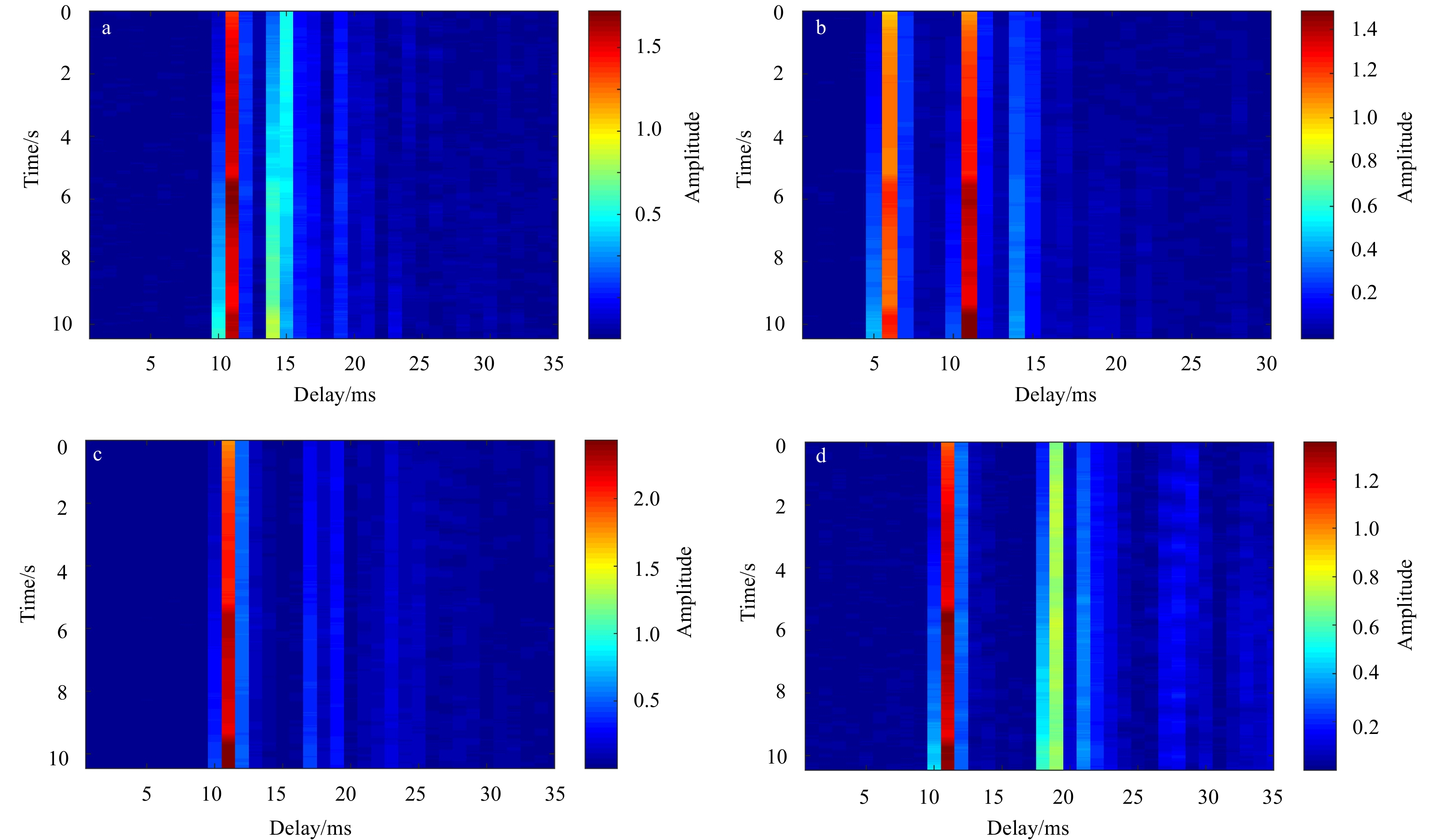
Figure 2 shows the channel impulse responses (CIRs) at different depths at range 500 m. Note that the self-recording hydrophone at 20 m could not work normally, so it is excluded when processing experimental data. It can be seen from Fig. 2 that (1) the channels show sparse feature and there are one or two distinct paths at different depths; (2) the channels are very stable throughout the whole signal duration with a small multipath spread (<10 ms); and (3) the first arrived path does not necessarily have the strongest power as shown in Fig. 2b.

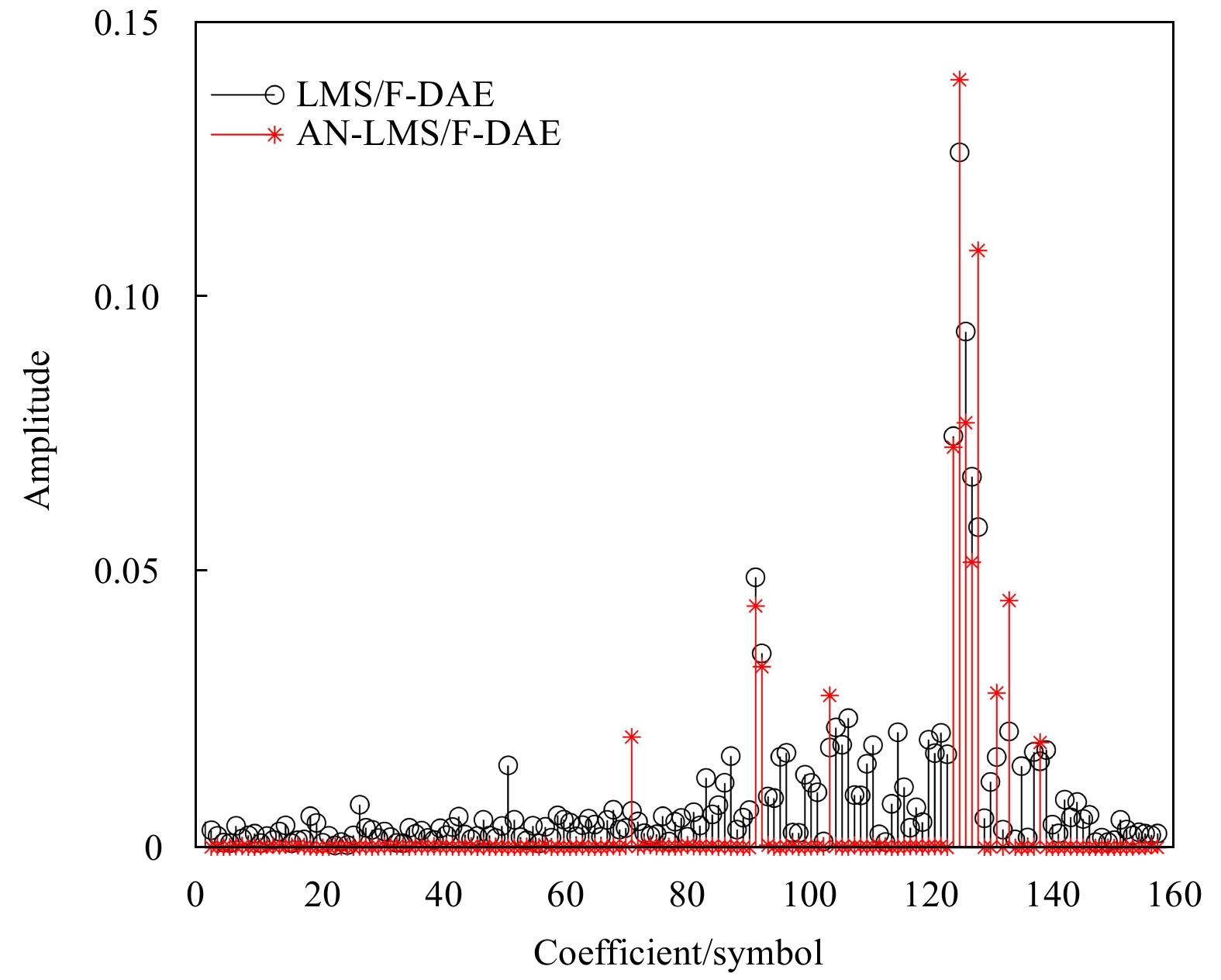
For experimental data at range 500 m, the SNR is relatively high because the distance is very close. In order to show the superior performance of the proposed algorithm at low SNR, additional ambient noise is superimposed to the received signal to reduce the SNR around 6.1 dB. The step size is set to be

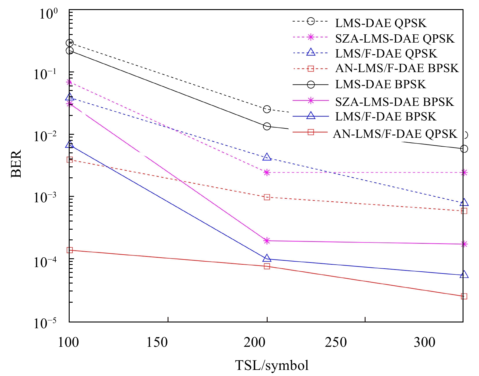
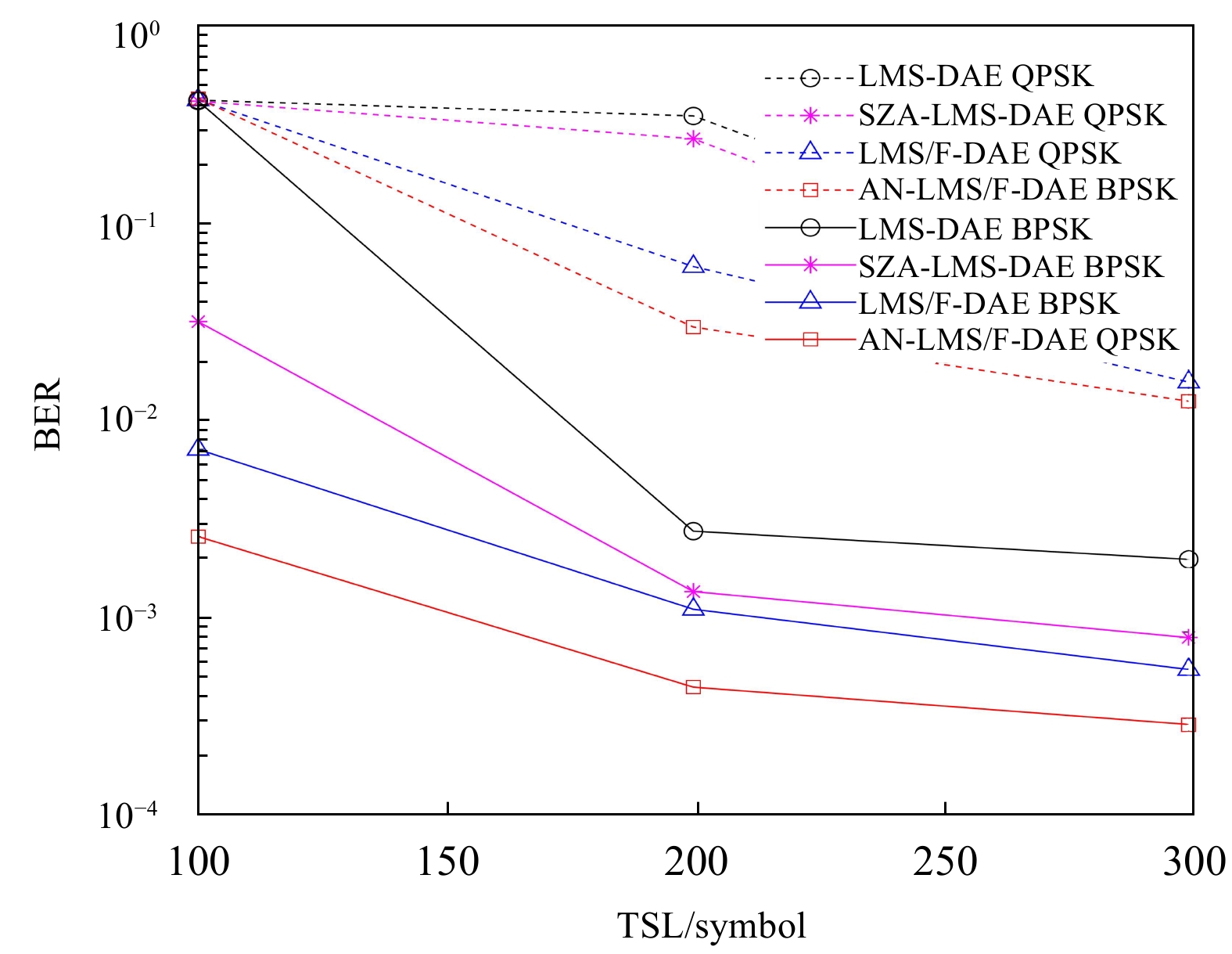
Then we compare the BER performance of LMS-DAE, SZA-LMS-DAE, LMS/F-DAE and AN-LMS/F-DAE under different training sequence lengths (TSLs) when BPSK or QPSK modulated signal is presented. It can be seen from the results shown in Fig. 4 that (1) the LMS/F-DAE has a lower BER and a better equalization performance compared with LMS-DAE; (2) when applying sparse constraints to LMS-DAE and LMS/F-DAE, the resulting SZA-LMS-DAE and AN-LM/S-DAE have better performance compared with their corresponding standard methods; and (3) AN-LMS/F-DAE has the fastest convergence speed as expected, and the equalization error of AN-LMS/F-DAE is comparable or slightly better than that of LMS/F-DAE. The reason can be explained as follows: AN-LMS/F-DAE imposes constraints on small coefficients to make them converge quickly, and does not impose constraints on large ones to ensure correct convergence to reduce equalization error, so it can achieve good performance in terms of convergence speed and BER performance.

Figure 5 shows the CIRs at different depths at range 4 km. Note that the self-recording hydrophone at 40 m could not work normally, so it is excluded when processing experimental data. The channels at range 4 km also show sparsity and they are also very stable just as shown in Fig. 2, but the structures of the channels are more complicated with much bigger multipath spread (>10 ms).

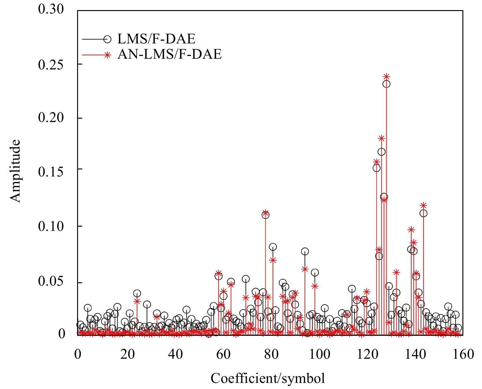
For experimental data at range 4 km, the SNR is very low. After going through a bandpass filter, the measured SNR is around 4.4 dB. The step size is set to be 0.002. In AN-LMS/F-DAE, we select

When the communication distance is 4 km, the trend of the BERs is demonstrated in Fig. 7. The results are consistent with those at range 500 m. The LMS/F-DAE outperforms the LMS-DAE counterpart in terms of convergence speed and equalization error. Although the performance improvement of AN-LMS/F-DAE is not as obvious as that in Fig. 4, it still outperforms LMS/F-DAE and shows the best performance.

In view of the sensitivity of the LMS-DAE to the input signal and SNR, this paper proposes an LMS/F-DAE which is capable of processing complex signals for UWA communication system. Take advantage of the sparse nature of the equalizer, a variable norm constraint is added to get the AN-LMS/F-DAE. It exerts constraints on small equalizer coefficients to converge quickly while exerting no constraints on large ones to ensure correct convergence. Therefore, it exhibits better performance in terms of convergence speed and equalization error. The experimental results of the 9th Chinese National Arctic Research Expedition confirm that compared with LMS/F-DAE, AN-LMS/F-DAE promotes the sparse level of the equalizer making most coefficients approach zero. Furthermore, it has better equalization performance than LMS/F-DAE.
We thank all participants of the Acoustic Communication Experiment of the 9th Chinese National Arctic Research Expedition for their assistance.
| [1] |
Berger C R, Zhou Shengli, Preisig J C, et al. 2010. Sparse channel estimation for multicarrier underwater acoustic communication: from subspace methods to compressed sensing. IEEE Transactions on Signal Processing, 58(3): 1708–1721. doi: 10.1109/TSP.2009.2038424
|
| [2] |
Brandwood D H. 1983. A complex gradient operator and its application in adaptive array theory. IEE Proceedings H Microwaves, Optics and Antennas, 130(1): 11–16. doi: 10.1049/ip-h-1.1983.0004
|
| [3] |
Chen Yilun, Gu Yuantao, Hero A O. 2009. Sparse LMS for system identification. In: 2009 IEEE International Conference on Acoustics, Speech and Signal Processing. Taipei, Taiwan: IEEE, 3125–3128
|
| [4] |
Duan Weimin, Tao Jun, Zheng Y R. 2018. Efficient adaptive turbo equalization for multiple-input-multiple-output underwater acoustic communications. IEEE Journal of Oceanic Engineering, 43(3): 792–804. doi: 10.1109/JOE.2017.2707285
|
| [5] |
Eksioglu E M. 2014. Group sparse RLS algorithms. International Journal of Adaptive Control and Signal Processing, 28(12): 1398–1412. doi: 10.1002/acs.2449
|
| [6] |
Eksioglu E M, Tanc A K. 2011. RLS algorithm with convex regularization. IEEE Signal Processing Letters, 18(8): 470–473. doi: 10.1109/LSP.2011.2159373
|
| [7] |
Falconer D, Ariyavisitakul S L, Benyamin-Seeyar A, et al. 2002. Frequency domain equalization for single-carrier broadband wireless systems. IEEE Communications Magazine, 40(4): 58–66. doi: 10.1109/35.995852
|
| [8] |
Freitag L, Koski P, Morozov A, et al. 2012. Acoustic communications and navigation under Arctic ice. In: 2012 Oceans. Hampton Roads, VA, USA: IEEE, 1–8
|
| [9] |
Guan Gui, Mehbodniya A, Adachi F. 2013a. Least mean square/fourth algorithm for adaptive sparse channel estimation. In: 2013 IEEE 24th Annual IEEE International Symposium on Personal, Indoor, and Mobile Radio Communications. London, UK: IEEE, 296–300
|
| [10] |
Guan Gui, Wei Peng, Adachi F. 2013b. Adaptive system identification using robust LMS/F algorithm. International Journal of Communication Systems, 27(11): 2956–2963
|
| [11] |
Lee Y, Cox D C. 1997. Adaptive DFE with regularization for indoor wireless data communications. In: IEEE Global Telecommunications Conference. Conference Record. Phoenix, AZ, USA: IEEE, 47–51
|
| [12] |
Li Haili, Ke Changqing, Zhu Qinghui, et al. 2019. Spatial-temporal variations in net primary productivity in the Arctic from 2003 to 2016. Acta Oceanologica Sinica, 38(8): 111–121. doi: 10.1007/s13131-018-1274-5
|
| [13] |
Li Weichang, Preisig J C. 2007. Estimation of rapidly time-varying sparse channels. IEEE Journal of Oceanic Engineering, 32(4): 927–939. doi: 10.1109/JOE.2007.906409
|
| [14] |
Liu Lu, Sun Dajun, Zhang Youwen. 2017. A family of sparse group lasso RLS algorithms with adaptive regularization parameters for adaptive decision feedback equalizer in the underwater acoustic communication system. Physical Communication, 23: 114–124. doi: 10.1016/j.phycom.2017.03.005
|
| [15] |
Mendel J M. 1991. Tutorial on higher-order statistics (spectra) in signal processing and system theory: theoretical results and some applications. Proceedings of the IEEE, 79(3): 278–305. doi: 10.1109/5.75086
|
| [16] |
Pelekanakis K, Chitre M. 2010. Comparison of sparse adaptive filters for underwater acoustic channel equalization/estimation. In: 2010 IEEE International Conference on Communication Systems. Singapore, Singapore: IEEE, 395–399
|
| [17] |
Pelekanakis K, Chitre M. 2013. New sparse adaptive algorithms based on the natural gradient and the l0 -norm. IEEE Journal of Oceanic Engineering, 38(2): 323–332. doi: 10.1109/JOE.2012.2221811
|
| [18] |
Stojanovic M, Catipovic J, Proakis J G. 1993. Adaptive multichannel combining and equalization for underwater acoustic communications. The Journal of the Acoustical Society of America, 94(3): 1621–1631. doi: 10.1121/1.408135
|
| [19] |
Tao Jun, An Liang, Zheng Y R. 2017. Enhanced adaptive equalization for MIMO underwater acoustic communications. OCEANS 2017-Anchorage. Anchorage, AK, USA: IEEE, 1–5
|
| [20] |
Vanbleu K, Ysebaert G, Cuypers G, et al. 2006. Adaptive bit rate maximizing time-domain equalizer design for DMT-based systems. IEEE Transactions on Signal Processing, 54(2): 483–498. doi: 10.1109/TSP.2005.861901
|
| [21] |
Vlachos E, Lalos A S, Berberidis K. 2012. Stochastic gradient pursuit for adaptive equalization of sparse multipath channels. IEEE Journal on Emerging and Selected Topics in Circuits and Systems, 2(3): 413–423. doi: 10.1109/JETCAS.2012.2214631
|
| [22] |
Walach E, Widrow B. 1984. The least mean fourth (LMF) adaptive algorithm and its family. IEEE Transactions on Information Theory, 30(2): 275–283. doi: 10.1109/TIT.1984.1056886
|
| [23] |
Wang Yanshuo, Huang Fei, Fan Tingting. 2017. Spatio-temporal variations of Arctic amplification and their linkage with the Arctic oscillation. Acta Oceanologica Sinica, 36(8): 42–51. doi: 10.1007/s13131-017-1025-z
|
| [24] |
Wu Feiyun, Tong Feng. 2013. Non-uniform norm constraint LMS algorithm for sparse system identification. IEEE Communications Letters, 17(2): 385–388. doi: 10.1109/LCOMM.2013.011113.121586
|
| 1. | Zehua Dai, Jinqiu Wu, Jingwei Yin, et al. DOA Estimation for Underwater Acoustic Array in Impulsive Noise Based on Adaptive Kernel Width Mixture Correntropy. IEEE Transactions on Geoscience and Remote Sensing, 2025, 63: 1. doi:10.1109/TGRS.2024.3509864 | |
| 2. | Ansuman Patnaik, Sarita Nanda. A switching norm based least mean Square/Fourth adaptive technique for sparse channel estimation and echo cancellation. Physical Communication, 2024, 67: 102482. doi:10.1016/j.phycom.2024.102482 | |
| 3. | Anand Kumar, Prashant Kumar. An improved sparsity‐aware normalized least‐mean‐square scheme for underwater communication. ETRI Journal, 2023, 45(3): 379. doi:10.4218/etrij.2022-0036 | |
| 4. | Ruibo Lei, Zexun Wei. Exploring the Arctic Ocean under Arctic amplification. Acta Oceanologica Sinica, 2020, 39(9): 1. doi:10.1007/s13131-020-1642-9 | |
| 5. | Syed Karimunnisa, Vadde Usha, Ashok Bekkanti, et al. Advanced patient's Heart Rate monitoring system using Cloud based Android system. 2021 Second International Conference on Electronics and Sustainable Communication Systems (ICESC), doi:10.1109/ICESC51422.2021.9532934 | |
| 6. | Dipanjan Dutta, Priya Ghosh, Ansuman Patnaik, et al. A Sparse Aware Arctangent Framework Based LHCAF Algorithm for System Identification. 2023 International Conference on Communication, Circuits, and Systems (IC3S), doi:10.1109/IC3S57698.2023.10169740 | |
| 7. | Yanan Tian, Xiao Han, Sergiy A. Vorobyov, et al. Improved Proportionate Least Mean Square/Fourth Based Channel Equalization for Underwater Acoustic Communications. 2023 IEEE 9th International Workshop on Computational Advances in Multi-Sensor Adaptive Processing (CAMSAP), doi:10.1109/CAMSAP58249.2023.10403523 |

Figures(7)

Supported by:
Beijing Renhe Information Technology Co. Ltd

Yanan Tian, Xiao Han, Jingwei Yin, Hongxia Chen, Qingyu Liu. An improved least mean square/fourth direct adaptive equalizer for under-water acoustic communications in the Arctic[J]. Acta Oceanologica Sinica, 2020, 39(9): 133-139. doi: 10.1007/s13131-020-1653-6

 DownLoad:


 DownLoad: