Ice sheet controls on fine-grained deposition at the southern Mendeleev Ridge since the penultimate interglacial

1. Introduction

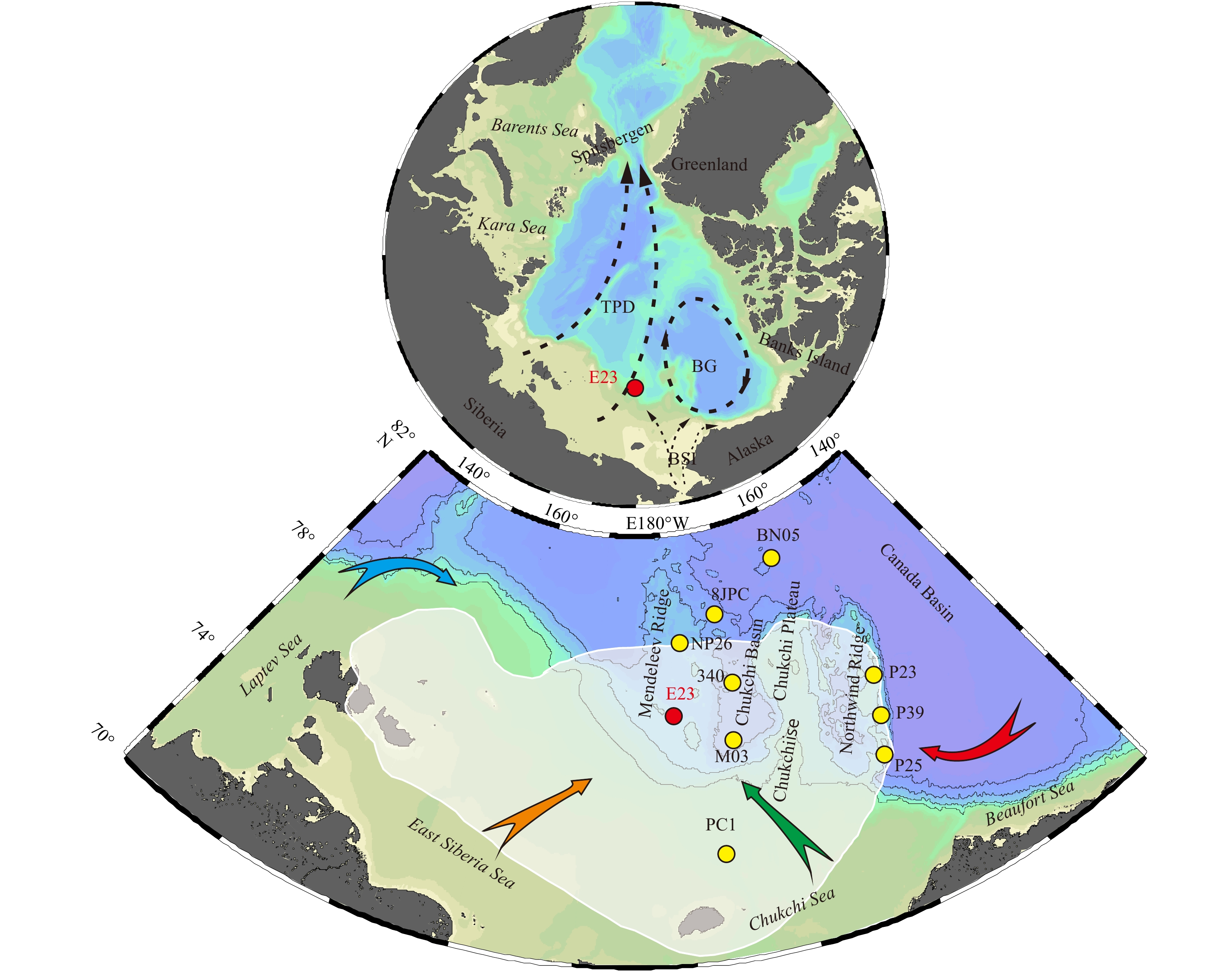
Since the Mid-Pleistocene Transition, Arctic ice sheets have been sensitive to global climatic changes with an eccentricity period of 100 ka, and have also been involved in a series of rapid climate changes, such as the Younger Dryas (YD) event (Berger and Jansen, 1994; Bond et al., 1997; Condron and Winsor, 2012). Planetary albedo, ocean circulation, and water balance are directly related to the Arctic ice sheets and its extended ice shelf (Clark et al., 1999, 2001; Zachos et al., 2001). The East Siberian Ice Sheet (ESIS) was proposed to have covered the southern Mendeleev Ridge in glacial periods, and sedimentary records near the ridge can reveal its evolution through time (Fig. 1; Jakobsson et al., 2016; Niessen et al., 2013; Stein et al., 2017).

Figure  1.  Geographic setting around the southern Mendeleev Ridge and location of Core E23. Core E23 (red circle) was the basis of this study; Cores PC1, M03, 340, NP26, 8JPC, BN05, P25, P23 and P39 (yellow circles) used for correlations are from Swärd et al. (2018), Wang et al. (2013), Stein et al. (2010), Polyak et al. (2004), Adler et al. (2009), Dong et al. (2017), Polyak et al. (2013), and Polyak et al. (2009), respectively. BG is Beaufort Gyre, TPD Transpolar Drift, BSI Bering Strait inflow (Talley et al., 2011). The bold red, green, brown, and blue arrows represent the proposed sources for kaolinite, chlorite, illite, and smectite, respectively (Stein, 2008; Wahsner et al., 1999).

DownLoad: Full-Size Img PowerPoint

Unlike glacial landforms, sedimentary records can provide a basis for ESIS identification and its spatial distribution through time (Polyak et al., 2007). Given the widespread sedimentary hiatuses associated with glacial expansion and poor preservation of older glacial landforms on continental shelves, it is difficult to determine the evolution of the ESIS (Dove et al., 2014). However, eroded sediments from shallow-water shelves or submarine highs were transported into deeper areas beyond the extent of glacial erosion. These sediments were deposited as glacial diamictons intercalated with normal pelagic, debris flow, and subglacial drainage system sediments (Dove et al., 2014; Jakobsson et al., 2010; Niessen et al., 2013; Polyak et al., 2001). Clay minerals can readily be entrained and transported long distances by icebergs, sea ice, and even currents, and have a unique provenance around the southern Mendeleev Ridge (Darby et al., 2011; Stein, 2008). Such sediments are a potential proxy of ice sheet expansion and retreat. In addition, numerous other proxies, such as foraminifera abundances, geochemical data, and grain size, are reliable environmental proxies. In this study, the evolution of the ESIS and changes in the local sedimentary environment over glacial-interglacial cycles were investigated mainly using the fine-grained sediments at the southern Mendeleev Ridge since the penultimate interglacial.

2. Background

Significant increases in ice-rafted debris (IRD) with a low carbonate content suggest there has been a Chukchi Sea shelf sediment source since Marine Isotope Stage 16 (MIS16) (Dove et al., 2014; Polyak et al., 2009; Stein et al., 2010). There are five sets of glaciogenic wedge-shaped sediments intercalated within well-stratified hemipelagic sediments on the East Siberian continental margin, indicating the ESIS has expanded at least five times since the Mid-Pleistocene (Niessen et al., 2013). Sedimentary cores near the Northwind Ridge confirmed that the latest expansion of the ESIS occurred in MIS4, but glacial landforms formed during MIS2 are also preserved on the western side of the Chukchi Rise (Polyak et al., 2001, 2009). The largest expansion of the ESIS may have occurred in MIS6, which is consistent with the development of other ice sheets around the Arctic Ocean (Jakobsson et al., 2016). The extended, thick, ice shelf grounded on seafloor at depths of deeper than 950 m on the southern Mendeleev Ridge (Niessen et al., 2013).

There is some evidence for glaciation on topographic highs of East Siberia, but no glacial landforms on the East Siberia inner shelf, apart from some buried channels that may be a subglacial drainage system (Colleoni et al., 2016; Dove et al., 2014). Thus, it is difficult to determine the southern boundary of the ESIS. To the north, an ice sheet on the Chukchi Sea shelf may have existed, and been followed by an isolated ice cap on the Chukchi Plateau (Dove et al., 2014; Jakobsson et al., 2005; Polyak et al., 2001, 2007). It has also been proposed that the ESIS might have covered the southern Mendeleev Ridge and almost the entire Chukchi Plateau and Northwind Ridge (Niessen et al., 2013). These inferences are mainly based on glaciogenic lineations or flutes with different directions that are found on the East Siberian margin and Chukchi borderland, which are considered to have been caused by fast-flowing ice streams (up to 1 600 m/a; Clark, 1993). These glacial landforms are abundant at the bottom of the Chukchi Rise, but not present at depths of <350 m (Dove et al., 2014). The spatial distribution of carbonate debris on the Chukchi Plateau and Northwind Ridge can also delineate the boundary between the ESIS- and Laurentide ice sheet (LIS)-originated icebergs, and is consistent with the direction of the glaciogenic lineations (Polyak et al., 2001; Dove et al., 2014). This boundary also appears to be recorded by the IRD distribution along the East Siberia margin, as there was no IRD deposition when the ESIS expanded (Ye et al., 2019). In general, ESIS expansion resulted in different depositional regimes, which provide the basis for tracking the evolution of the ESIS with sediment records.

3. Materials and methods

A gravity sediment core (ARC7-E23; hereafter E23) with a length of 354 cm was recovered from the southern Mendeleev Ridge at a water depth of 1 107 m during the Seventh Chinese Arctic Expedition in 2016. The core contains no obvious turbidites, and subsequent analysis indicated that Mn and Ca contents and other sedimentary characteristics are comparable with neighboring cores. The core location was either covered by or very close to the proposed ESIS during glacial periods (Fig. 1).

The core was split lengthwise into two halves, and X-ray fluorescence (XRF) scanning was undertaken to obtain high-resolution Mn and Ca content data with an Itrax Core Scanner at the Key Laboratory of Submarine Geosciences (KLSG), Ministry of Natural Resources, Hangzhou, China. The analyses were conducted using the methodology of Löwemark et al. (2011), with a resolution of 5 mm and an exposure time of 5 s using a Mo X-ray tube. Analytical precision was firstly assessed by the emitted energy at a testing signal intensity of more than 29 000 counts per second, and then checked with the risk function with a mean-square-error of less than 8 counts per second.

After XRF scanning, the core was sampled in 2 cm increments. All samples were freeze-dried and weighed. About 10 g of each sample was soaked in the deionized water for 2 d. The samples were then washed through a 63 μm sieve. The residues were dried at 40°C and the weight of the coarse-grained fraction was used to estimate the amount of IRD (Stein et al., 2010).

The fine fraction (<63 μm) of each sample was used for clay mineral analysis. The carbonate and organic material were removed at room temperature with 1 mol/L HCL and 30% H₂O₂, respectively. Clay fractions (<2 μm) were obtained by settling (Liu et al., 2010 and references therein). Each sample was transferred to two slides by wet smearing. One of the air-dried sample slides was prepared for qualitative clay mineral identification. The other slide was treated with ethylene glycol in a desiccator for at least 36 h at 35°C. Clay minerals were analyzed with a PANalytical diffractometer over a 2θ range of 3° to 35° at steps of 0.0167° at the KLSG. Semi-quantitative estimates of peak areas for the main clay minerals were carried out on the ethylene glycol treated sample data using MDI Jade 6.0 software. The percentage of clay minerals was calculated according to Biscaye (1965). The 17 Å and 10 Å peaks were used for the smectite and illite calculations, respectively. Kaolinite (3.58 Å) and chlorite (3.54 Å) peaks were identified to calculate their proportions from the 7 Å kaolinite + chlorite peak (Biscaye, 1965). The analytical precision was assessed by 15 replicate analyses, which yielded a standard deviation of less than 3%.

For grain size analysis, about 0.3 g of wet bulk sediment was decalcified at room temperature using 1 mol/L HCL, followed by two rinsing steps, and organic material removal with 30% H₂O₂. Sediment disaggregation was undertaken by adding 100 mL of 0.5 Na₄P₂O₇·10H₂O. The entire sample was used for the grain size analysis, and ultrasonicated for 1 min before measurement with a Malvern Mastersizer 2000 at the KLSG. Each sample was analyzed in 65 bins between 0.02 μm and 2 000 μm. All grain size components were calculated in volume percentages (vol.%), following the size scale of Blott and Pye (2001) (and references therein): clay (<4 μm), silt (4–63 μm), and sand (63–2 000 μm). The end-member (EM) modeling algorithm proposed by Dietze et al. (2012) was used for grain size data decomposition. The algorithm is based on principal component analysis and the factor analysis, and can provide EMs directly comparable to the scale of the original data, which readily allows identification of the underlying sedimentary processes or sources. Mathematically, an EM can be defined as either a concrete or an idealized population of one or more variables with a characteristic frequency distribution (Dietze et al., 2012). Analytical precision was assessed by 11 replicate analyses, which yielded a standard deviation that was mostly less than 1% and rarely up to 6%. Samples were re-analyzed if the standard deviation was more than 10%.

Planktic foraminifera abundance was determined on the greater than 150 μm fraction. For accelerator mass spectrometry (AMS) ¹⁴C dating, 7–10 mg of well-preserved specimens of Neogloboquadrina pachyderma-sin were picked from six samples at depths of 0–2 cm, 6–8 cm, 10–12 cm, 60–62 cm, 76–78 cm, and 82–84 cm. AMS ¹⁴C ages were determined at Beta Analytic, Florida, USA. The conventional ¹⁴C age was used without a reservoir correction, which is poorly understood in Arctic Ocean sediments. While not particularly accurate, this approach provided general age constraints on the youngest sediments.

4. Results

4.1 General stratigraphy

The most prominent sedimentary characteristic in Core E23 is coloration, and in general the core comprises brown and gray layers, similar to cores reported elsewhere from the western Arctic Ocean (Fig. 2; Adler et al., 2009; Polyak et al., 2004; Stein et al., 2010). Four distinct brown layers form first-order color cycles and were named B1–B4 from top to bottom, which correspond to high Mn contents (Fig. 2). Another type of color layer, characterized by a light yellowish to pinkish coloration, was called the pink–white (PW) layers, which corresponds to a high carbonate content (Fig. 2; Clark et al., 1980; Polyak et al., 2004; Stein et al., 2010). Three main Ca peaks in Core E23 are associated with brown Layers B1, B2, and B3, but not all are represented by PW layers (Fig. 2). Since the Mid-Pleistocene, three carbonate layers have been deposited across the western Arctic Ocean, which are named PW1, PW2, and PW3 (Stein et al., 2010). Based on coloration, Ca contents, and its spatial relationship to brown Layers, PW3 was identified at a depth of 60 cm in Core E23, but the other two PW layers were not identified (Fig. 2).

Figure  2.  Generalized stratigraphy and clay mineralogy of the Core E23. Brown lithostratigraphic layers are indicated by Layers B1, B2, B3 and B4 (Polyak et al., 2004). PW3 means pink-white layers (Stein et al., 2010). Arrows annotated with numbers are the AMS ¹⁴C ages. Horizontal gray bars indicate the interglacial periods based on Cores NP26 and 8JPC (Adler et al., 2009; Polyak et al., 2004).

DownLoad: Full-Size Img PowerPoint

The coarse-grained sediment content representative of IRD (>63 μm) ranges from 0% to 36%, with an average of 2.3%, and displays a close relationship to the sediment color cycles. In general, high IRD contents characterize brown layers and IRD contents are nearly 0% in gray layers (Fig. 2). Planktic foraminifera (>150 μm) can be observed at several discrete depth intervals, with high abundances in brown layers and nearly zero abundances in gray layers. Abundant planktic foraminifera (up to 5 434 ind./g) only exist at depths of 0–20 cm and 52–82 cm within the brown Layers B1 and B2, respectively. However, the brown Layers B3 and B4 contain no foraminifera. Neogloboquadrina pachyderma-sin picked for AMS ¹⁴C dating show the youngest conventional age (4 140 a) at a depth of 0–2 cm and oldest age (>43 500 a) at a depth of 82–84 cm, with no age reversals (Fig. 2).

4.2 Clay minerals

Illite is the dominant clay mineral in Core E23, with an average content of 62%, followed by chlorite and kaolinite with average contents of 20% and 12%, respectively. Smectite contents have an average of 7%. In the depth profile, kaolinite uniformly reaches a lowest content of about 8% in each gray layer, but has high or low peaks in content in the brown layers. In the brown Layer B2, kaolinite rapidly increases to its highest content of 26% and then decreases gradually. Kaolinite contents are negatively correlated with illite contents over the first-order color cycles (Fig. 2). Illite reaches a maximum content of about 65% in almost every gray layer, and has relatively low contents in brown layers. Kaolinite content is positively correlated with IRD content. Each peak of kaolinite, including the highest peak in the brown Layer B2, corresponds to an IRD peak. When kaolinite contents are lowest, the IRD contents are nearly 0%.

Smectite shows similar trends as kaolinite, generally having high contents in brown layers and low contents in gray layers, but smectite and kaolinite contents are not correlated in sub-layers (Fig. 2). In the brown Layer B2, smectite reaches its highest content of 15%. There is a negative correlation between smectite and kaolinite contents in a thin gray layer dividing brown Layers B3 and B4. The last gray layer at the bottom of the core has a higher smectite content than the brown Layer B1. Using kaolinite as a reference, chlorite contents fluctuate over the first-order color cycles with two different patterns. In the brown layers, chlorite shows similar trends as kaolinite. In the gray layers, chlorite and kaolinite do not correlate. The poorest correlation occurs in the gray layer dividing brown Layers B2 and B3, where chlorite reaches its highest content of 23%.

4.3 Grain size components and end-members

Grain size components in the sediments vary significantly from 0%–41% sand, 31%–68% silt, and 21%–69% clay, with averages of 3%, 49% and 48%, respectively. Only the sand content correlates with the first-order color cycles, with higher contents in brown layers and low contents in gray layers (Fig. 3). Clay and silt dominate most samples and can have high contents in both brown and gray layers.

Figure  3.  Grain size components and end-members (EMs). Mean variable- and sample-wise coefficients of determination (r²) with different end-members (a and b), which were obtained using the algorithm proposed by Dietze et al. (2012). Dominant modes of the three end-member model at 3 μm, 16 μm and 149 µm (c). Grain size components (GSC) calculated in volume percentages (vol.%) following the size scale of Blott and Pye (2001) (and references therein), and the end-member scores. Horizontal gray bars indicate the interglacial periods (d).

DownLoad: Full-Size Img PowerPoint

Different EM models were performed to decompose the grain size data. The first step was to check the data validity, which allows 0 to be set as the only value for weight transformation. The mean variable-wise (grain size class) coefficient of determination (r²) between the original (X) and modeled dataset (X′) increases sharply from 55% to 72%, with the number of EMs increasing from two to three (Fig. 3). The coefficient at a grain size of about 10 μm has been significantly improved, but that at a grain size of 500 μm is still poor. In contrast, the mean sample-wise (sediment depth) r² decreased from 88% to 86%. When the number of EMs increases from three to four, the mean variable-wise r² continues to increase smoothly to 78%. In fact, as the number of EMs increases, the mean variable-wise r² becomes higher, while the mean sample-wise r² decreases gradually until the number of EMs reaches seven.

Combining the statistical parameters with the grain size features of modern Arctic Ocean sediments (Clark and Hanson, 1983; Darby et al., 2009; Nürnberg et al., 1994), produces an equilibrium state between the modeled and sample grain size results when a three EM model is used. This yields EMs 1–3 with dominant modes at 3 µm, 16 µm and 149 µm, and each EM represents 40%, 35% and 25% of the total variance, respectively. More than one additional minor mode was modeled in each EM that has subordinate importance. EM1 consists mainly of clay and contains a large amount of well-sorted fine silt. EM2 is dominated by well-sorted silt (10–63 μm). In addition to sand, EM3 contains two robust minor modes at 2 µm and 21 µm, representing significant amounts of clay and silt, respectively. As such, EM3 is very poorly sorted.

EM scores provide quantitative information on the EMs in sample space, representing the degree to which an EM contributes to each sample (Dietze et al., 2012). EM1 fluctuates over the first-order color cycles, with very high scores in gray layers and relatively low scores in brown layers (Fig. 3). Specifically, EM1 reaches near 0% at the depths where sand contents are highest and EM1 is highest at the depths where sand contents are 0%. EM2 shows a weak negative correlation with EM1 in the sub-layers, but no apparent fluctuations over the first-order color cycles. EM3 changes markedly over the first-order color cycles, is very low in all gray layers, and is highest in the brown layers where EM1 is lowest.

5. Discussion

5.1 Age model on an orbital timescale

After calibration by absolute dating methods such as ¹⁴C, ¹⁰Be, amino acid racemization (AAR), and optically stimulated luminescence (OSL), Mn stratigraphy provides a convenient correlation method for Arctic Ocean sediments since the Mid-Pleistocene (Adler et al., 2009; Jakobsson et al., 2003; Spielhagen et al., 2004). There is a good correspondence between Mn contents and oxygen isotopes (LR04), but several disadvantages exist when using Mn stratigraphy, such as diagenetic redistribution of Mn, terrigenous dilution, and bioturbation (Jakobsson et al., 2000; Löwemark et al., 2012, 2014; März et al., 2011).

In terms of stratigraphic characteristics, Core E23 shows excellent consistency with other cores from the Mendeleev Ridge, Chukchi Basin, and Chukchi borderland (Fig. 1; Polyak et al., 2004, 2009; Stein et al., 2010). Each brown layer was confirmed to represent a warm interglacial/interstadial period, with a high stand of sea-level, and enhanced primary productivity that promoted Mn enrichment (Jakobsson et al., 2000; MacDonald and Gobeil, 2012). Unlike other Arctic Ocean areas, IRD deposition at the southern Mendeleev Ridge and Chukchi borderland occurred mostly in interglacial/interstadial periods, rather than in glacial/stadial periods (Ye et al., 2019). In Core E23, high IRD contents directly correspond to brown layers, representing interglacial/interstadial periods (Fig. 2).

AMS ¹⁴C dates show that sediments at the top of Core E23 were deposited in the Holocene, and no sediment loss occurred during core recovery. The deposition of the first brown layer B1 can be assigned to MIS1, and the second brown Layer B2 to MIS3, based on the age model for nearby Core NP26 (Polyak et al., 2004). Brown Layers B3 and B4 and the intervening carbonate layer, were initially assigned to MIS5 (Polyak et al., 2004). AAR dating has further refined this to MIS5a (interstadial) as recorded in Core 8JPC (Adler et al., 2009). As such, we infer that the age of basal sediments in Core E23 are MIS5b (ca. 85 ka), and the corresponding sedimentation rate was about 4.2 cm/ka. Calcareous foraminifera shells are typically absent in sediments deposited after MIS7 due to enhanced dissolution, although that occurred in MIS5a at the southern Mendeleev Ridge, probably due to its proximity to the continental margin where lateral transport of organic matter was significant (Polyak and Jakobsson, 2011; Wang et al., 2013).

By correlating the four brown layers, the positions of MIS1, MIS3, and MIS5a can be broadly determined. Their boundaries, defined according to Mn, IRD, and foraminifera abundances, are close to those defined by oxygen isotopes, if there has been no substantial diagenetic redistribution (Jakobsson et al., 2000). Although some features of this tentative age model, such as the position of the deglaciation, are still challenging to define, correlations between Core E23 and nearby cores provide a reasonable age model.

5.2 Clay mineral sources

Clay minerals that originate from the continents are largely deposited on the Arctic Ocean shallow shelves or continue to be transported to the deep sea across the shallow shelf (Darby et al., 2011; Nürnberg et al., 1994; Wahsner et al., 1999). A series of shallow shelves semi-surround the southern Mendeleev Ridge, serving as potential provenances with a diagnostic assemblage of clay minerals (Bazhenova et al., 2017; Bischof and Darby, 1997; Stein et al., 2010). Based on the distribution of clay minerals in Arctic surface sediments, the highest illite contents in the Arctic Ocean characterize the East Siberia Sea shelf and the highest chlorite contents are in the Chukchi Sea (Fig. 1; Stein, 2008; Wahsner et al., 1999). The highest contents of smectite and kaolinite can be found on shelves far from the southern Mendeleev Ridge. The nearest shallow shelf to the southern Mendeleev Ridge is in the Laptev Sea, where the smectite content is second only to that in the Kara Sea (Stein, 2008). In addition, the Beaufort Sea is rich in kaolinite, and the Canadian Archipelago may also have an important role in kaolinite supply, based on dirty sea ice observations (Darby et al., 2011).

The fine-grained deposition at the southern Mendeleev Ridge records dramatic changes in provenance over glacial-interglacial cycles as in Core E23 (Figs 1 and 4). During MIS2 and MIS4, an illite-rich source was dominant, followed by a chlorite-rich source. In the interglacial/interstadial, the contribution from the illite-rich source decreased rapidly, and contributions from kaolinite- and smectite-rich sources increased abruptly. This change was most significant in MIS3, followed by MIS5a, and was weaker in MIS1. Presently, a weak and isolated Beaufort Gyre (BG) in combination with a strong Transpolar Drift (TPD) is associated with the positive phase of the Arctic Oscillation (AO), which is associated with fast passage of Laptev Sea ice across the Arctic Ocean and retention of Arctic Canada sea ice in the BG (Funder et al., 2011). When the AO shifts into a negative phase, the Mendeleev Ridge is strongly affected by the BG (Steele et al., 2008). AO-like conditions may have also occurred during the previous interglacial/interstadial, resulting in smectite enrichment when the TPD expanded. If this is not the case, then kaolinite enrichment is expected. An isotopic mixing model has shown that, although sediments derived from Arctic Canada increased during interglacial periods, Siberian sediment input always dominated, even in the PW layer (Bazhenova et al., 2017).

Figure  4.  Ternary diagram with end members of illite, kaolinite, and smectite. Colored symbols indicate samples from MIS1 to MIS5b in Core E23. Dark arrows indicate the input of kaolinite and smectite in the interglacial/interstadial periods. a–f are the clay mineralogies for different areas in the Arctic Ocean (Wahsner et al., 1999).

DownLoad: Full-Size Img PowerPoint

The variable changes in chlorite contents are of important significance, as these are closely related to its source. During glacial periods, the East Siberia Sea shelf and part of the Chukchi Sea shelf were covered by the proposed ESIS (Dove et al., 2014; Niessen et al., 2013), and chlorite-rich sediments should have been transported to the southern Mendeleev Ridge along with illite. However, the illite source was stable and strong, whereas the chlorite source increased rapidly in the early stage of glacial periods and then decreased rapidly, reflecting a lack of a sustainable supply (Fig. 2). When the Bering Strait opened and sea-level rose during the deglaciation, chlorite transport was facilitated from the northern Bering Sea shelf to the Chukchi Sea shelf, and chlorite deposition increased and fluctuated according to the strength of Bering Strait inflow (Deschamps et al., 2018; Yamamoto et al., 2017). However, sea-level is not considered to have been high enough to open the Bering Strait during MIS3.

5.3 Sediment transport dynamics

It is not easy to identify a specific transport process for one type of clay mineral. For example, smectite in central Arctic surface sediments cannot solely be attributed to sea ice transport from the Laptev Sea (Stein, 2008; Wahsner et al., 1999). However, a similar grain size component indicative of sea ice transport will always be extracted from surface sediments, regardless of location (Darby et al., 2009; Reimnitz et al., 1998).

Amongst the three grain size EMs in Core E23, EM1 is well-sorted and dominated by clay and fine silt (<10 μm). In previous studies, it was considered that the grain size spectrum of EM1 represents sea ice sediments entrained by suspension freezing (Clark and Hanson, 1983; Darby et al., 2009; Nürnberg et al., 1994). EM1 does not show any correlation with the clay mineralogy over glacial-interglacial cycles, but within a specific period (e.g., MIS3), the smectite content correlates with EM1, indicating that sea ice from different sources was vigorously mixed during transport process, as is presently the case (Darby et al., 2011). As such, only when sea ice transport is dominant in a specific region, can the clay mineralogy in sediments be effectively indicated (Fig. 3).

The grain size spectrum of EM3 also shows a significant amount of clay and fine silt (<10 μm), while the main component is sand that is greater than 100 μm in grain size. The variation of EM3 in the depth profile is the same as that of the IRD, and shows an increasing trend in the Holocene. Anchor ice as another way of sea ice entrainment, is characterized by sediments with a variable grain size, reflecting the shelf sediment from which it is obtained (Darby et al., 2009). Modern observations show that anchor ice transport occurs mainly in the Canadian Arctic, and that most of these sediments are <30 μm in grain size, but occasionally are >100 μm (Darby et al., 2011). As such, we speculate that the primary transport process indicated by EM3 is anchor ice, but we cannot entirely rule out iceberg transport. West of the Laptev Sea, remnants of the Eurasian Ice Sheet (EAIS) have been reported to have existed in early MIS3 (Fig. 5; Jakobsson et al., 2014; Mangerud et al., 2004; Spielhagen et al., 2004). A similar situation may have also characterized the Canadian Arctic, where some remnants of the LIS existed that produced icebergs. EM3 exhibits very significant glacial-interglacial cycles, and correlates with kaolinite contents, indicating that anchor ice or icebergs originating from the Canadian Arctic were a key transport process for kaolinite.

Figure  5.  Correlation between the ESIS expansion and sediment inputs revealed by clay minerals in Core E23 and ε_Nd values for sediments in Core 340 (Bazhenova et al., 2017) and ice streams around Spitsbergen (Jakobsson et al., 2014). Sea-level was taken from Spratt and Lisiecki (2016; low-resolution) and Siddall et al. (2003; high-resolution). Brown lithostratigraphic layers are indicated by B1, B2, B3 and B4 (Polyak et al., 2004). PW3 means pink-white layer (Stein et al., 2010). Horizontal gray bars indicate the interglacial periods.

DownLoad: Full-Size Img PowerPoint

EM2 is characterized by sortable silt, which accounts for 35% of the explained variance. Although only sparse data are available for the Arctic, reported velocity measurements of the slope boundary current along the Eurasian margin range from 1 cm/s to 5 cm/s (Coachman and Barnes, 1963). A 5 cm/s current corresponds to a shear velocity of 0.3 cm/s, which is sufficient for the transportation of fine particles in suspension (Darby et al., 2009). In terms of its grain size spectrum, EM2 is likely to represent the bottom currents that winnowed away part of the fine-grained material and left behind the coarse-grained mode of 16 μm, which differs from the deposition of winnowed silt on the Chukchi-Alaskan shelf (Darby et al., 2009; Dipre et al., 2018). Recent studies of sediment cores and geophysical observations have identified past current-controlled erosion-deposition regimes in the deep Arctic Ocean, such as north of the Chukchi margin (Dipre et al., 2018; Hegewald and Jokat, 2013). The East Siberian provenance characterized by illite was covered by the proposed ESIS during the glacial periods when sea-level fell by nearly 120 m and most Siberian shelves were exposed (Fig. 5; Niessen et al., 2013; Spratt and Lisiecki, 2016). A key question is how these illite-rich sediments were transported to the southern Mendeleev Ridge and deposited. Glacial landforms along the East Siberian margin suggest strong ice stream activity, which removed sediments from shelves or highs and deposited them onto the slope by debris flows (Dove et al., 2014; Swärd et al., 2018). This is similar to the subglacial drainage system under the modern Antarctic ice sheet, which flushes out sediments from the shelves (Ashmore and Bingham, 2014; Dong et al., 2017). In this process, bottom currents along the slope may play a key transport role, such as winnowing of the fine-grained sediments from the slope to the southern Mendeleev Ridge. However, there are no distinct glacial-interglacial cycles for these bottom currents indicated by EM2, and EM2 appears to fluctuate at a higher frequency.

5.4 ESIS expansion

The glacial landforms, IRD distribution, and clay mineralogy changes indicate that the ESIS was a significant control on deposition at the southern Mendeleev Ridge. In Core E23, IRD (including carbonate debris), kaolinite, and smectite contents were high in MIS5a, indicating that material from the Canadian Arctic and Laptev Sea reached the southern Mendeleev Ridge. This scenario is also supported by the low ε_Nd sediment values in nearby Core 340, representing dolomite input from the Canadian Arctic (Figs 1 and 5; Bazhenova et al., 2017). In MIS4, IRD almost disappeared, kaolinite contents decreased to their lowest level, and smectite contents decreased significantly. In contrast, a nearby core (BN05) in the central Arctic Ocean records its highest kaolinite, smectite, and IRD contents at this time (Dong et al., 2017). It is likely that a large number of icebergs derived from the LIS or EAIS were imported into the western Arctic Ocean, but could not reach the southern Mendeleev Ridge due to the presence of the ESIS (Fig. 5).

The expansion of Arctic ice sheets was not always synchronous (Ehlers and Gibbard, 2007). Since the Mid-Pleistocene, the EAIS may have expanded most extensively in MIS6, while the LIS reached its maximum extent in MIS2 (England et al., 2009; Spielhagen et al., 2004). Niessen et al. (2013) proposed that the maximum extent of the ESIS covered the southern Mendeleev Ridge, Chukchi Plateau, and Northwind Ridge, but did not specify when this occurred. Based on the clay mineralogy in Core E23 and IRD records in Cores P23, P25 and P39 on the Northwind Ridge (Polyak et al., 2009, 2013), the ESIS should have expanded northward and covered the Northwind Ridge in MIS4, but it is not clear whether this is the largest extent of the ESIS since the Mid-Pleistocene. However, it is clear that the Northwind Ridge and Chukchi Platform were not covered by the ESIS in MIS2. A large number of icebergs were imported from the LIS, which resulted in abundant IRD deposition and the NW-SE-trending glacial lineations on the Northwind Ridge and Chukchi Plateau (Dove et al., 2014; Jakobsson et al., 2005; Polyak et al., 2001, 2007). Meanwhile, the lowest kaolinite and near-zero IRD contents are recorded in Core E23. Changes in ε_Nd values in Core 340 (Fig. 5), near-zero IRD contents in the nearby Cores M03 and 340, and 13 ka deposition of unfossiliferous, overcompacted sediment characterized the Chukchi Rise at this time and indicate the presence of an ice sheet (Niessen et al., 2013; Polyak et al., 2001). Therefore, we speculate that compared with MIS4, the ESIS retreated significantly and may have become an ice cap in MIS2, but still controlled the southern Mendeleev Ridge and Chukchi Rise.

6. Conclusions

The source of fine-grained sediment deposition at the southern Mendeleev Ridge has changed significantly since the penultimate interglacial. During glacial periods, fine-grained sediments were mainly imported from the East Siberia Sea and Chukchi Sea, while during interglacial/interstadial periods, sediment supply from the Canadian Arctic and Laptev Sea became more significant.

The fine-grained deposition was first controlled by the extent of the ESIS. Previous studies considered that the last expansion of the ESIS occurred in MIS4, but the sedimentary record in the present study show that the ESIS-extended ice shelf still covered the southern Mendeleev Ridge and Chukchi Rise in MIS2. When the ESIS-extended ice shelf completely covered the southern Mendeleev Ridge, almost all sediments from the Canadian Arctic and Laptev Sea were blocked, and deposition was dominated by fine-grained sediments from the East Siberia and Chukchi Sea shelves.

After the ESIS retreat, the depositional regime over the southern Mendeleev Ridge was mainly controlled by the relative strength of the BG and TPD, and also regulated by the types of transport processes. Sea ice entrained by suspension freezing had multiple sources and was strongly mixed during the transport process, and so there is no correspondence between sea ice and smectite deposition. However, the sources of anchor ice or icebergs are relatively simple and, to some extent, can be indicated by kaolinite deposition, even when the TPD expanded. The climate conditions in MIS3 were apparently the most suitable for fine-grained sediment deposition at the southern Mendeleev Ridge, due to the multiple transport processes and improved circulation around the ridge.

Acknowledgements

We thank the crew members and scientists onboard R/V Xuelong for their support during the 7th Chinese Arctic Expedition, and Polyak L for his valuable suggestions on the age model. We also thank Li Qi for his technical support with clay mineral analysis.