Comparisons of passive microwave remote sensing sea ice concentrations with ship-based visual observations during the CHINARE Arctic summer cruises of 2010–2018
State Key Laboratory of Coastal and Offshore Engineering, Dalian University of Technology, Dalian 116024, China
2.
MNR Key Laboratory for Polar Science, Polar Research Institute of China, Shanghai 200136, China
3.
Institute of Atmospheric and Earth Sciences, University of Helsinki, Helsinki 00014, Finland
Funds:
The National Major Research High Resolution Sea Ice Model Development Program of China under contract No. 2018YFA0605903; the National Natural Science Foundation of China under contract Nos 51639003, 41876213 and 41906198; the High-tech Ship Research Project of China under contract No. 350631009; the National Postdoctoral Program for Innovative Talent of China under contract No. BX20190051.
In order to apply satellite data to guiding navigation in the Arctic more effectively, the sea ice concentrations (SIC) derived from passive microwave (PM) products were compared with ship-based visual observations (OBS) collected during the Chinese National Arctic Research Expeditions (CHINARE). A total of 3 667 observations were collected in the Arctic summers of 2010, 2012, 2014, 2016, and 2018. PM SIC were derived from the NASA-Team (NT), Bootstrap (BT) and Climate Data Record (CDR) algorithms based on the SSMIS sensor, as well as the BT, enhanced NASA-Team (NT2) and ARTIST Sea Ice (ASI) algorithms based on AMSR-E/AMSR-2 sensors. The daily arithmetic average of PM SIC values and the daily weighted average of OBS SIC values were used for the comparisons. The correlation coefficients (CC), biases and root mean square deviations (RMSD) between PM SIC and OBS SIC were compared in terms of the overall trend, and under mild/normal/severe ice conditions. Using the OBS data, the influences of floe size and ice thickness on the SIC retrieval of different PM products were evaluated by calculating the daily weighted average of floe size code and ice thickness. Our results show that CC values range from 0.89 (AMSR-E/AMSR-2 NT2) to 0.95 (SSMIS NT), biases range from −3.96% (SSMIS NT) to 12.05% (AMSR-E/AMSR-2 NT2), and RMSD values range from 10.81% (SSMIS NT) to 20.15% (AMSR-E/AMSR-2 NT2). Floe size has a significant influence on the SIC retrievals of the PM products, and most of the PM products tend to underestimate SIC under smaller floe size conditions and overestimate SIC under larger floe size conditions. Ice thickness thicker than 30 cm does not have a significant influence on the SIC retrieval of PM products. Overall, the best (worst) agreement occurs between OBS SIC and SSMIS NT (AMSR-E/AMSR-2 NT2) SIC in the Arctic summer.
As an intuitive and sensitive indicator of global climate change, Arctic sea ice plays an important role in the global climate system (Vihma, 2014; Overland et al., 2015; Sui et al., 2017). Under the background of global warming, the Arctic has warmed twice as fast as the global average. This phenomenon, which is widely known as the “Arctic Amplification Effect” (Pithan and Mauritsen, 2014; Cohen et al., 2014), has led to the drastic melting of Arctic sea ice. Since the beginning of continuous satellite observations of sea ice in October 1978, numerous studies have shown that the sea ice extent, area, concentration, and thickness, as well as the proportion of multi-year ice, have decreased significantly in the Arctic region (Comiso, 2012; Lei et al., 2015; Chen and Zhao, 2017; Wang et al., 2019b). The rapid melting of Arctic sea ice undoubtedly brings unprecedented convenience to navigation and in situ scientific investigation in the Arctic. However, the complex ice conditions of the Arctic Ocean also represent great difficulties and threats to these activities. It is therefore crucial to grasp the temporal and spatial distribution of Arctic sea ice as accurately as possible, both for studies of global climate change, forecast of Arctic sea ice conditions, and especially for Arctic navigation in ice zones (Khon and Mokhov, 2010; Khon et al., 2017).
As an important parameter characterizing the sea ice condition, sea ice concentration (SIC) is of great significance for Arctic navigation and sea ice management. Because the Arctic sea ice cover area is vast, the geographical location is remote, and conducting field observations is difficult, remote sensing observation represents an essential source of data for grasping the Arctic sea ice conditions (McIntire and Simpson, 2002). Passive microwave (PM) remote sensing has become the preferred method for the long-term continuous acquisition of large-scale polar sea ice horizontal distribution data. This is due to the excellent long-wave penetration characteristics of PM, which gives it the ability to distinguish sea ice from the cloud, and the ability to conduct continuous observations of sea ice under polar night conditions.
The PM SIC is obtained by inputting the acquired brightness temperatures (Tb) data into retrieval algorithms. Therefore, even if the same PM sensor is used, the final results of SIC retrievals can be quite different because different algorithms combine Tb data at different frequencies and for different polarization components. Many scholars have evaluated the performances of the PM algorithms by comparing the differences between the sea ice area, extent and concentration derived from the various algorithms (Comiso et al., 1997; Ivanova et al., 2014; Hao and Su, 2015).
However, this is not sufficient to determine the reliability and validity of SIC retrieved by these algorithms. The most direct and effective way to evaluate the merits and demerits of SIC retrieval algorithms is to validate them by using field SIC data. The commonly used method is to regard SIC data obtained by means of ship-based visual observations (OBS), helicopter or unmanned aerial vehicle aerial photography (AP) in ice zones as ground truth value, and compare them with SIC retrieved by different sensors and algorithms (Worby and Comiso, 2004; Knuth and Ackley, 2006). Ozsoy-Cicek et al. (2009) found that compared with the National Snow and Ice Data Center (NSIDC) AMSR-E product, the National Ice Center (NIC) ice charts obtained from high-resolution satellite images exhibited better consistency with OBS data, and that the AMSR-E product tended to underestimate ice conditions during Antarctic summer due to its relatively low resolution. Ozsoy-Cicek et al. (2011) reported that the correlation between OBS data and PM data in the marginal ice zones (MIZ) of West Antarctica, and over most of the sea-ice zones of East Antarctica was less than that in the 90°W region, and that the extent of Antarctic sea ice estimated by AMSR-E data was 1×10⁶–2×10⁶ km2 less than that estimated by NIC data. Beitsch et al. (2015) compared more than 21600 OBS SIC around Antarctica with seven kinds of PM SIC retrieved by five algorithms based on SSM/I-SSMIS and AMSR-E sensors. Their results showed that the Bootstrap (BT) algorithm was the best choice both for the SSM/I-SSMIS comparison and the AMSR-E comparison. Shi et al. (2015) used CHINARE-2012 helicopter AP and SAR images to evaluate the PM SIC based on the “HY-2” scanning radiometer in the Arctic. They reported that the SIC from the “HY-2” products in the central Arctic Ocean was 16% higher than that obtained by AP, and its root-mean-square difference with SAR derived data was between 8.57% to 12.34%. By comparing the SIC extracted from ship-based monitoring images with SSMIS NASA TEAM (NT) and AMSR-2 Sea Ice Climate Change Initiative (SICCI) SIC data, Wang et al. (2019a) reported that the SIC obtained from SSMIS and AMSR-2 were 9.5% and 9.9% higher than the OBS SIC respectively, and that the overestimation of SSMIS and AMSR-2 SIC increased to 12% and 16.4% respectively, in areas where the OBS SIC was less than 15%. Meanwhile, the underestimation of SSMIS and AMSR-2 SIC were 4.4% and 8.9% in areas where the OBS SIC was greater than 75%.
In order to apply PM data to Arctic ice management and navigation guidance more effectively, the acquisition of a large quantity of historical field observations from many cruises is needed to verify and evaluate the accuracy of PM products. In this paper, numerous OBS SIC data collected during the five Chinese National Arctic Research Expeditions (CHINARE) cruises were compared with the six long time series PM SIC products commonly used. The PM sensors, SIC retrieval algorithms and products, OBS data, data preprocessing and comparison methods are first introduced in Section 2. The results of these comparisons are introduced in Section 3, while Section 4 is dedicated to the evaluation of the performances of the PM SIC products in the Arctic summer, and to a discussion on the limitations of the visual observations and methods used in this paper. Finally, Section 5 provides conclusions.
2.
Data and methods
2.1
PM sensors
In 2003, SSMIS replaced SSM/I for installation on the Defense Meteorological Satellite Program (DMSP) F-16 satellite and its successor. SSMIS augments the imaging channel of SSM/I by several atmospheric sounding channels, but still retains the ability of SSM/I to record Tb, whose 19, 22, 37 and 85 GHz (91 GHz for SSMIS) imaging channels are associated with SIC retrieval (Beitsch et al., 2015). The 91 GHz channel, as a high frequency channel, can provide higher spatial resolution. Using SSMIS as well as earlier SSM/I and SSMR data, SIC products with a spatial resolution of 25 km × 25 km or 12.5 km × 12.5 km can be used for global climate change analysis from 1978 to present.
AMSR-E was launched onboard the Aqua satellite on May 2, 2002, and ceased operation on December 4, 2011. The time coverage of its data ranges from June 18, 2002, to October 4, 2011. Like the DMSP satellites, Aqua also orbits the Earth in a near-polar solar synchronous orbit. AMSR-2, as the successor to AMSR-E, was launched onboard the Global Change Observation Mission for Water-1 (GCOM-W1) satellite by the Japan Aerospace Exploration Agency (JAXA) on May 1, 2012. The main mission of AMSR-2 is to detect the earth’s water and energy cycle. The scanning angle of incidence is 55° and provides a 1 450-km swath width at the Earth’s surface (Beitsch et al., 2014). Compared with AMSR-E, AMSR-2 includes two extra channels of 7.3 GHz, which can be used to mitigate the effects of the radio frequency interference (RFI). The size of its main reflector is increased to 2.0 m, which leads to smaller footprints and improves the spatial resolution for different frequencies (Beitsch et al., 2014). Compared with SSMIS, AMSR-E and AMSR-2 mainly present the advantage of having a higher spatial resolution (Table 1). At present, SIC products based on AMSR-E and AMSR-2 with spatial resolution up to 3.125 km × 3.125 km are provided by the University of Bremen (UB).
For AMSR-E and AMSR-2 datasets, AMSR-2 Tb are converted to equivalent AMSR-E Tb after regression analysis of AMSR-2 Tb and AMSR-E Tb, so that the same algorithm can be used with data from these two sensors without any significant impact on the SIC retrievals (Meier and Ivanoff, 2017). From here on, the combined SIC data based on AMSR-E and AMSR-2 measurements will be referred to as AMSR.
2.2
SIC retrieval algorithms and products
The PM SIC data used in this paper are derived from six long time series SIC products which are commonly used and are still being regularly updated. These products use the NT, BT and Climate Data Record (CDR) algorithms for SSMIS-based data, and the BT, enhanced NASA-Team (NT2) and ARTIST Sea Ice (ASI) algorithms for AMSR-based data. An overview of these SIC retrieval algorithms and products is given in Table 2.
The basic principle of the NT algorithm is to use the 19 GHz vertical and horizontal, and 37 GHz vertical polarization Tb to calculate polarization ratios (PR) and gradient ratios (GR) to identify the open water, first-year ice and multi-year ice, so as to retrieve SIC (Smith, 1996).
The basic principle of the BT algorithm is to identify open water and sea ice by using the differences of polarization Tb between the 37 GHz vertical and horizontal channels, and between the 37 GHz and 19 GHz vertical channels, in order to retrieve SIC (Smith, 1996).
CDR algorithm is a combination of the NT and BT algorithms, which aims to utilize the advantages of both algorithms to generate a more precise SIC field (Peng et al., 2013).
NT2 algorithm is an improved algorithm designed to mitigate the problems inherent to the NT algorithm. NT2 calculates PR and GR in the same way as NT, but, in order to avoid the influence of snow cover on the ice type identification, PRR is calculated and the high frequency (89 GHz for AMSR) vertical and horizontal channels polarization Tb are used to calculate ∆GR to estimate the surface effect (Markus and Cavalieri, 2000).
ASI algorithm was developed from the Arctic Radiation and Turbulence Interaction Study (ARTSIST) in 1998. The ASI algorithm only uses the difference between the polarization Tb of the 89 GHz horizontal and vertical channels to retrieve SIC, and uses the low frequency Tb as a weather filter to filter out the misestimates of SIC caused by atmospheric water vapor in some MIZ and in the ice-free area (Spreen et al., 2008). Compared with other high-frequency algorithms using 89 GHz Tb, the ASI algorithm can achieve similar results without additional input data (Kern et al., 2003). However, the precondition to determine the tie point for the ASI algorithm is to make the results of SIC retrievals closest to those obtained by the BT algorithm (Spreen et al., 2008). As a result, the result of SIC retrievals from the ASI algorithm depends on the retrieval accuracy of the BT algorithm.
2.3
Ship-based visual OBS data
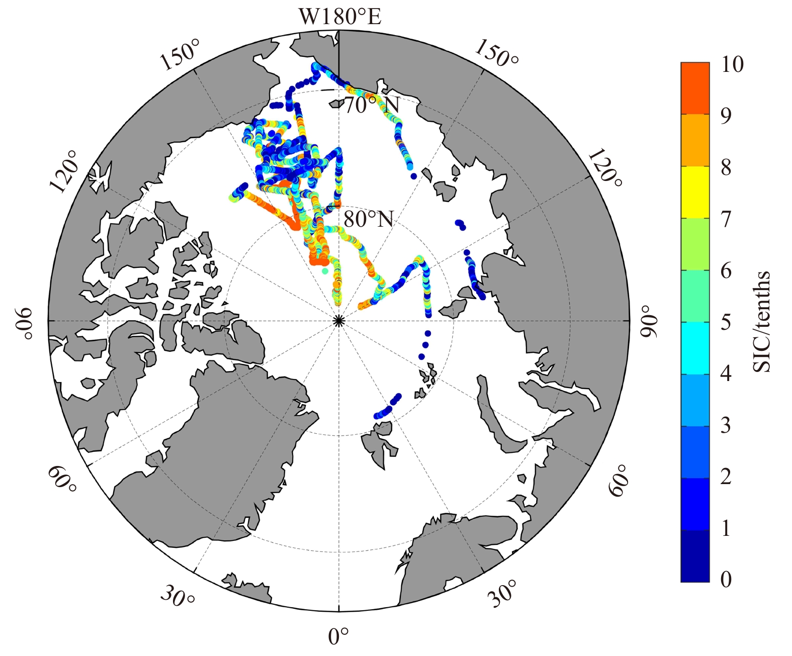
The ship-based visual OBS data used in this paper come from the CHINARE cruises of 2010, 2012, 2014, 2016 and 2018, and contain 3 667 observations altogether. The distribution of the OBS SIC obtained during these cruises is shown in Fig. 1. An overview of information on the visual OBS data obtained during these cruises is provided in Table 3.
Figure
1.
The distribution of the OBS SIC obtained during the CHINARE cruises used in this paper.
Onboard observations of sea ice were carried out when the R/V Xuelong icebreaker was sailing in ice zones, according to the SIC visual observation methodology recommended by the Antarctic Sea Ice Processes and Climate (ASPeCt) protocol (Worby et al., 1999). The ASPeCt protocol was originally designed for Antarctic sea ice observations and has since been expanded to the Arctic region (Polashenski et al., 2015; Istomina et al., 2015). A standard set of observations is conducted by an observer on the ship’s bridge, recording the ship’s position as well as total ice concentration (Ct), and an estimate of the concentration (Ca, Cb and Cc), thickness (Tha, Thb and Thc), floe size (Fa, Fb and Fc, recorded with code), topography, and snow cover of the three dominant ice thickness categories (recorded as Type a, b and c in the CHINARE cruises) within a radius of approximately 1 km of the ship (Worby et al., 1999). The three dominant ice thickness categories are defined as those with the greatest concentration, and the thickest of these is defined as the primary ice type (Worby et al., 1999). There may be times when only one or two different ice categories are present in which case only the primary, or primary and secondary, classifications are defined (Worby et al., 1999). For the CHINARE cruises, the sea ice observation codes were adjusted for Arctic sea ice and the coverage rate of melt ponds was also recorded. The duration of a single observation was 5–10 min. When the sailing speed was less than 6 kn, the ice condition was observed and recorded every hour; when the sailing speed was greater than 6 kn, the ice condition was observed and recorded every half hour. When the expedition carried out short-term (within one day) or long-term (several days or more) ice camp observations, the R/V Xuelong stopped sailing and no visual observation of sea ice was recorded.
Because the OBS SIC is measured to the nearest 10%, there is a rounding error as high as 5% (Worby and Comiso, 2004). In addition, the subjective nature of the observations makes it difficult to quantify differences between the OBS SIC obtained by different observers. However, experiments have shown that when observations are conducted by different observers simultaneously, the overall SIC difference between observers rarely exceeds 10% (Worby and Comiso, 2004). Weissling et al. (2009) also suggested that the absolute error of SIC observations following the ASPeCt protocol is below 10%.
2.4
Data preprocessing and comparison methods
The OBS SIC represents the average SIC, measured in tenths, within an elliptically-shaped area with a semi-minor axis of about 1 km, observed periodically for 5–10 min. The PM SIC provides the day-average SIC of each grid cell, in percent. The maximum grid resolution of the PM SIC products used in this study is 3.125 km × 3.125 km, and the minimum is 25 km × 25 km. As the temporal and spatial resolution of OBS data are much higher than those of the PM data and plotting each raw value may result in too scattered results with little evident relationship, direct comparison between the two kinds of data can be problematic (Worby and Comiso, 2004; Knuth and Ackley, 2006; Beitsch et al., 2015). In order to minimize problems related to the inconsistent spatial and temporal of the two kinds of data, the OBS and PM SIC are first daily- and spatially-averaged. Specifically, for each OBS SIC, the PM SIC of the nearest grid cell at the same date was selected, following which, the daily average of all OBS SIC and corresponding PM SIC were calculated and compared. This method is similar to the method described by Beitsch et al. (2015) to use daily-average along-ship-track SIC values. The R/V Xuelong icebreaker did not always sail at a uniform speed in the ice zones, and the ship would slow down under severe ice conditions. For example, when sailing in an area with numerous ice ridges, the R/V Xuelong may even cruise at a speed of only a few hundred meters per hour. As the maximum grid cell size of the PM products used here is up to 25 km × 25 km, it is inevitable that multiple OBS SIC correspond to the same PM SIC (Fig. 2). The method used in Beitsch et al. (2015) is similar to calculating the arithmetic average of PM SIC and that of OBS SIC.
Figure
2.
A hypothetical example of the distribution of OBS SIC and PM SIC in one day. The direction of the arrow is the direction of travel. The red dots represent the positions of the OBS SIC. The squares represent the PM SIC grid cells, and the blue squares with numbers represent the grid cells where the red dots fall in. The size of the squares is equal to the spatial resolution of the PM product.
The average method in this paper consists in calculating the arithmetic average of PM SIC and the weighted average of OBS SIC, as shown in Eqs (1) and (2):
as shown in Fig. 2, where CPM and COBS are the average of PM SIC and OBS SIC within one day, Ci and Cij are, respectively, the PM SIC and OBS SIC of the corresponding PM grid cell, i is the serial number of the PM grid cell and j is the serial number of OBS SIC within the same PM grid cell along the direction of sailing.
After the preprocessing of the two kinds of data, the correlation coefficients (CC), biases and root mean square deviations (RMSD) are calculated between each daily mean PM SIC and OBS SIC, as the basis for evaluating the retrieval accuracy of each product.
CC were used to measure the linear correlation between PM SIC and OBS SIC, while biases were used to qualitatively and quantitatively evaluate potential misestimates of PM SIC. Lastly, RMSD were used to measure the deviation between PM SIC and OBS SIC. The relationship between RMSD and bias is as follows:
where SDD is the standard deviation of the deviations between PM SIC and OBS SIC, which is used to measure the dispersion of deviations themselves. Therefore, RMSD takes into account both bias and SDD.
3.
Results
3.1
Overall comparisons between PM SIC and OBS SIC
After the preprocessing of the two types of data, 124 groups of daily average SIC data were obtained. The results of daily mean PM SIC and daily mean OBS SIC are presented in Fig. 3 and summarized in Table 4.
Figure
3.
Comparison of daily mean SIC between OBS data and PM data for each product (a–f). The black solid lines represent the equality “y = x”. The black dashed lines represent the linear fit of the data points. The blue and red dashed lines represent the 95% lower and upper confidence interval. Also shown are the equations of the linear fit, coefficients of determination (R2), and the significance levels (P).
As can be seen from Fig. 3a, overall, SSMIS-NT tends to underestimate SIC, with low OBS SIC (0%–20%) often corresponding to no sea ice being recorded by PM product. SSMIS-BT (Fig. 3b) and SSMIS-CDR (Fig. 3c) tend to overestimate SIC but also show an inability to detect sea ice when OBS SIC is low (0%–15% for SSMIS-BT and 0%–25% for SSMIS-CDR), whereas when OBS SIC>75%, these products often yield SIC values of 100%. A good agreement between AMSR-BT (Fig. 3d) SIC and OBS SIC exists when OBS SIC<30%, whereas with increasing OBS SIC, AMSR-BT tends to overestimate SIC, and when OBS SIC>75%, AMSR-BT also usually yields a value of 100%. AMSR-NT2 (Fig. 3e) tends to underestimate SIC when OBS SIC<15% and overestimate SIC when OBS SIC>30%. AMSR-ASI (Fig. 3f) tends to underestimate SIC or is unable to detect sea ice when OBS SIC<40%, and overestimate SIC when OBS SIC>40%. When OBS SIC>80%, it tends to consider the whole observation area as completely covered by sea ice (i.e., SIC=100%). It is noteworthy that, except SSMIS-NT, SIC is never underestimated when OBS SIC is more than 70%.
PM SIC products compare badly with observations for low and high SIC mainly due to the low spatial resolution of PM SIC products. It may be difficult for PM SIC algorithms to identify sea ice from large-area open water when SIC is low, and to identify leads and openings from sea ice when SIC is high. Most PM algorithms calibrate the atmosphere or use weather filters for the water vapor and other components misjudged as sea ice, and doing so tends to cut off the low SIC values (Peng et al., 2013; Beitsch et al., 2015). Therefore, when SIC is low, PM algorithms tend to underestimate SIC or even may not observe sea ice at all.
As shown in Table 4, SSMIS-NT presents the largest CC value (0.95), and AMSR-NT2 the smallest (0.89). The bias between SSMIS-NT SIC and OBS SIC is smallest and negative (−3.96%), which indicates an overall underestimation of SIC results from this product, whereas AMSR-NT2 presents the largest bias (12.05%). The RMSD is the smallest for SSMIS-NT SIC (10.81%) and the largest for AMSR-NT2 (20.15%).
3.2
Comparisons between PM SIC and OBS SIC under different ice conditions
According to the WMO (1970) description of the relationship between SIC and ice conditions, and referring to the definition by Shibata et al. (2013) of the relationship between sea ice cover and ship navigation difficulty, SIC was classified here into three categories: 0%–30%, 30%–70%, and 70%–100%. These three categories correspond to mild (easy to navigate), normal (somewhat difficult to navigate) and severe ice condition (very difficult to navigate), respectively. Among the daily average SIC data, 35, 54 and 34 samples corresponded to these three ice conditions, respectively. The CC, bias, and RMSD between PM SIC and OBS SIC were then calculated for each of the three categories and for each product and are shown in Fig. 4.
Figure
4.
Statistical results of CC (a), bias (b), and RMSD (c) between PM SIC and OBS SIC for each product under the three categories of ice condition.
Compared with the overall comparisons, Fig. 4a shows that the CC between PM SIC and OBS SIC are significantly reduced. The CC between PM SIC (except for AMSR-ASI) and OBS SIC are lowest under the severe ice condition, ranging from 0.24 (SSMIS-CDR) to 0.69 (AMSR-ASI). This means that the overestimation of SIC under severe ice conditions may be greater than the underestimation under mild ice conditions. Under the mild ice condition, the CC between PM SIC and OBS SIC are higher and close to the values under the normal ice condition. CC values range from 0.57 (AMSR-ASI) to 0.77 (AMSR-BT) under mild ice condition, against 0.64 (SSMIS-BT) to 0.74 (AMSR-BT) under normal ice condition.
Figure 4b shows that the biases between SSMIS-NT SIC and OBS SIC are negative under all ice conditions, i.e., the SSMIS-NT product underestimates SIC under any ice condition. Under the mild ice condition, the biases are relatively low, ranging from −5.31% (AMSR-ASI) to 3.73% (SSMIS-BT), whereas they increase a lot (except for SSMIS-NT) under the normal ice condition, with values ranging from −5.04% (SSMIS-NT) to 18.80% (AMSR-NT2). Under the severe ice condition, the biases range from −1.79% (SSMIS-NT) to 12.47% (AMSR-BT).
As shown in Fig. 4c, the RMSD are largest for all the PM products under the normal ice condition, which range from 12.91% (SSMIS-NT) to 25.90% (AMSR-BT). Under the mild ice condition, the RMSD range from 8.52% (AMSR-BT) to 15.10% (AMSR-NT2). Lastly, under the severe ice condition, the RMSD range from 8.68% (SSMIS-NT) to 14.59% (AMSR-BT).
3.3
Influences of floe size and ice thickness on the PM SIC retrieval
As stated in Section 2, not only the total ice concentration, but also the ice concentration, ice thickness, floe size and other information pertaining to the three dominant ice categories (Types a, b and c) were recorded as part of the OBS dataset. Here, the influences of floe size and ice thickness on the SIC retrievals of different PM products were evaluated by calculating the daily weighted average of the floe size code and ice thickness along the ship track, defined in Eqs (4) and (5):
where F is the floe size code, Th is the ice thickness (cm), C is the ice concentration (in tenths); subscript character a, b and c represent the three ice types, t represents the total ice; n is the quantity of sets of records in one day, and i is the index number of the sets of records within one day.
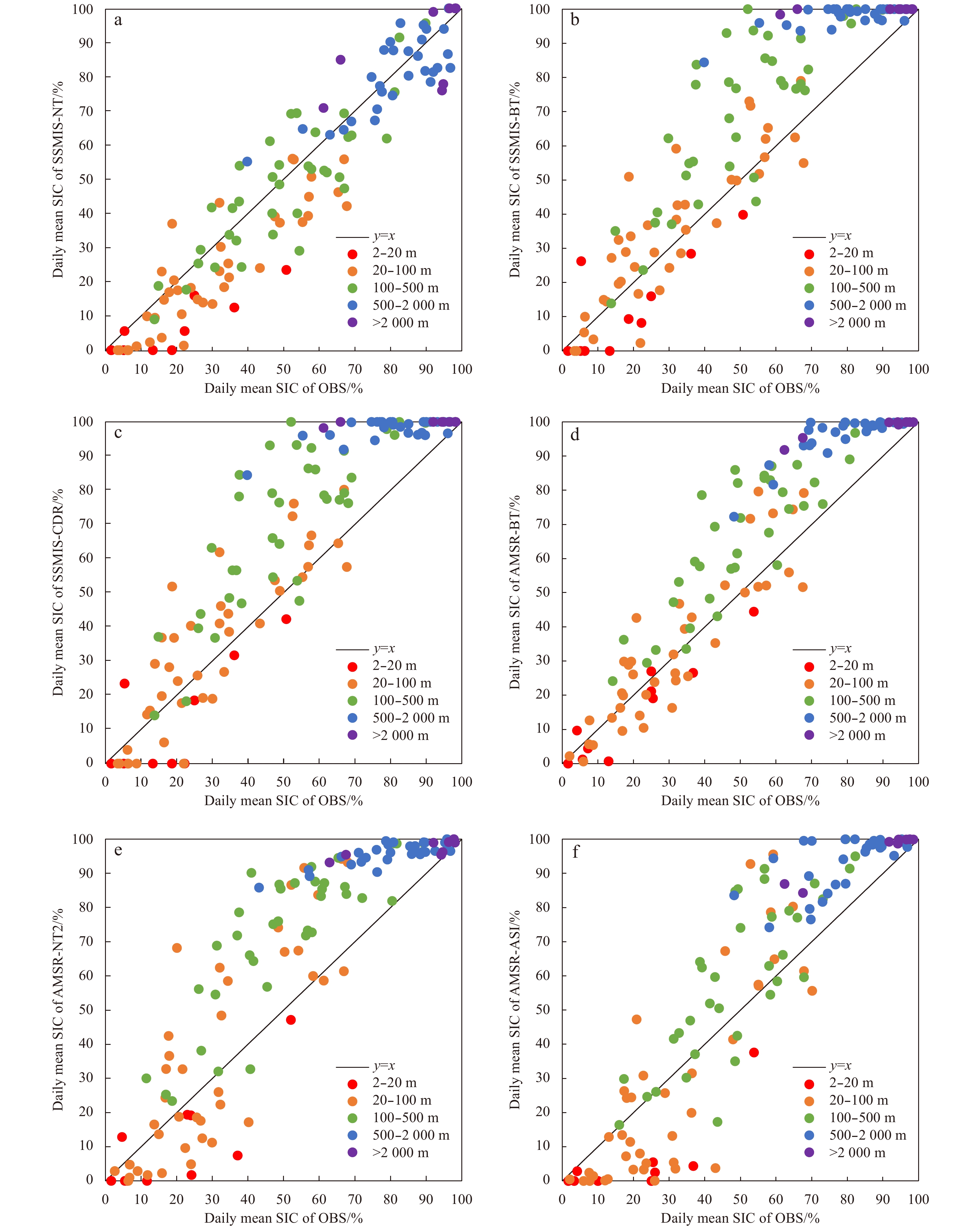
The results presented in Fig. 3 are then shown according to their floe size type and ice thickness category in Figs 5 and 6, respectively.
Figure
5.
The effect of floe size on SIC retrieval for each PM product (a–f). The black solid lines represent the equality “y = x” and the different colors represent the different floe sizes.
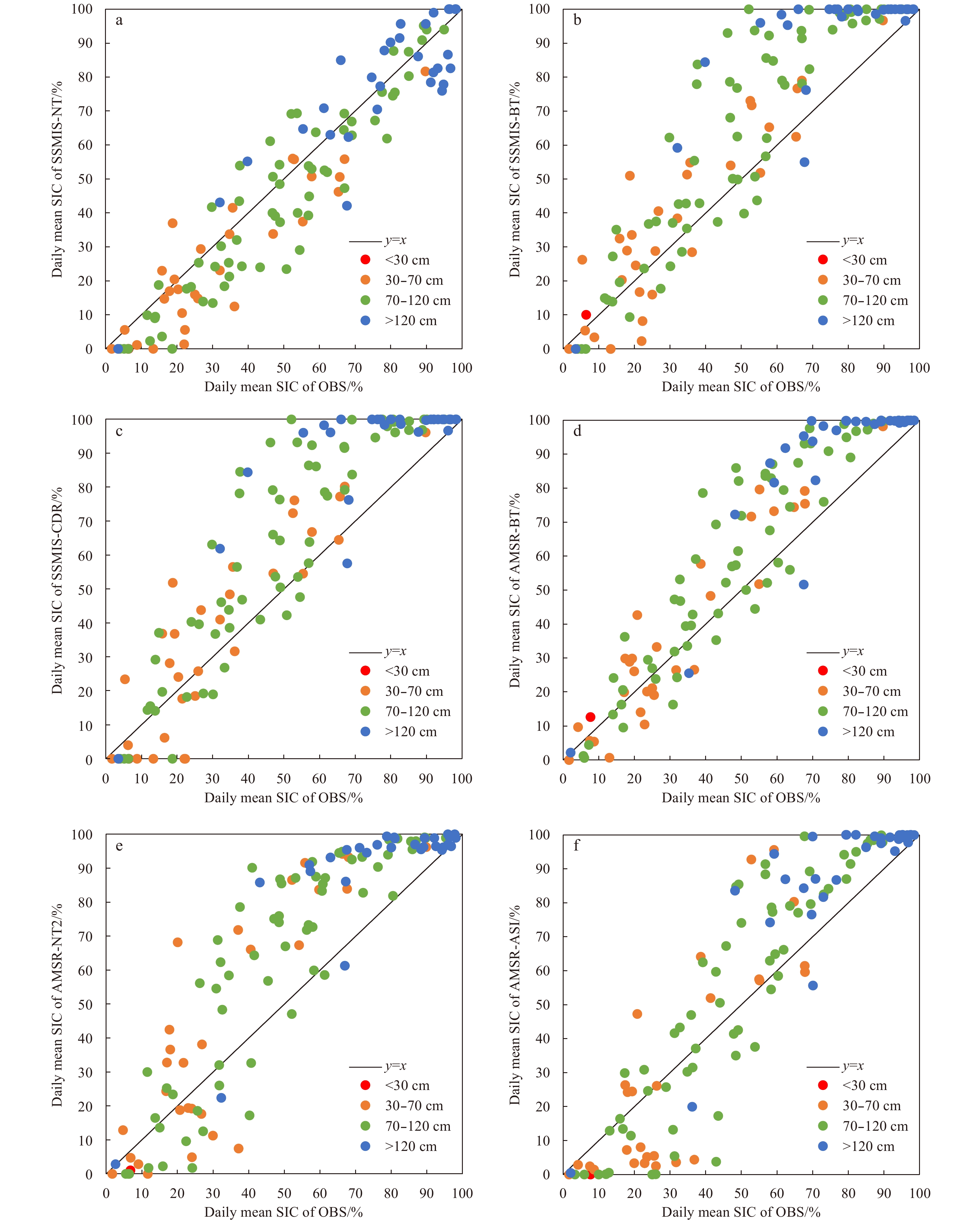
Figure
6.
The effect of ice thickness on SIC retrieval for each PM product (a–f). The black solid lines represent the equality “y=x” and the different colors represent the different ice thickness.
As can be seen from Fig. 5, floe size affects the SIC retrievals in that most of the PM products tends to underestimate (overestimate) SIC when the floe size is smaller (larger). This may be due to the large footprints of the PM channels, which result in the low spatial resolution, failing to distinguish small floe size sea ices from open water and to effectively identify leads and openings from ice zones when the floe size is large. The floe size associated with underestimation of SIC is <100 m for SSMIS-NT, and <20 m for SSMIS-BT, SSMIS-CDR, AMSR-NT2, and AMSR-ASI. However, no such influence exists for AMSR-BT. In contrast, SIC tends to be overestimated when floe size exceeds 100 m for SSMIS-BT, SSMIS-CDR, AMSR-BT and AMSR-NT2, and 500 m for AMSR-ASI. When the floe size is larger than 500 m, SSMIS-BT and SSMIS-CDR usually judge the whole observation area to be completely covered by sea ice (i.e., SIC=100%), whereas the large floe size does not appear to affect SSMIS-NT results. When the floe size is between 20 m and 100 m for AMSR-NT2, and between 20 m and 500 m for AMSR-ASI, SIC shifts from being underestimated to being overestimated with increasing OBS SIC.
Based on the WMO (1970) sea ice classifications, the ice thickness is classified into four grades, <30 cm, 30–70 cm, 70–120 cm and >120 cm.
Contrary to the ice floe case, the results of Fig. 6 show no clear relationship between ice thickness and PM SIC values. There is, however, only one sample with ice thickness less than 30 cm, which makes it impossible to judge the possible effect of thin ice on PM SIC retrievals. Many studies have investigated the influence of thin sea ice on the SIC retrievals of PM algorithms (Kwok et al., 2007; Ivanova et al., 2015), and Heygster et al. (2014) pointed out that the existence of thin ice has a great influence on the horizontal polarization channels. In particular, they found that among the six products, SSMIS-NT, which uses the lowest-frequency algorithm, is the most affected by thin ice, while AMSR-ASI is the least affected because only 89-GHz high-frequency data are used. The penetration depth of the main frequencies used for SIC retrievals is less than 30 cm (Mathew et al., 2009), and Heygster et al. (2014) reported that brightness temperatures are influenced by ice thickness below 18 cm (89 GHz) and 50 cm (1.4 GHz) and that PM SIC retrievals are degraded for ice thickness below 0.17 m and 0.33 m, for the 89 GHz and 1.4 GHz frequencies, respectively, i.e. the higher the frequency, the smaller the influence of thin ice on the SIC retrievals is. To our knowledge, few studies have investigated the influence of thick ice on PM SIC retrievals, and the results of Fig. 6 suggest that sea ice thickness thicker than 30 cm does not have a significant impact on PM SIC values.
4.
Discussion
4.1
Performance evaluation of the PM SIC products in the Arctic summer
An overview of the overall performances (defined as a summary of the statistical properties) of the 6 PM products is provided in Table 5. With regards to the results delineated in Section 3, most of the PM products tend to underestimate SIC when SIC is low or the floe size is smaller, and to overestimate SIC when SIC is high or the floe size is larger.
Table
5.
Overview of the overall performances of the 6 PM products in the summer Arctic
PM Product
CC
Bias/%
RMSD/%
Resolution
Comment
SSMIS-NT
0.95
−3.96
10.81
25 km × 25 km
best linear correlation, unique negative bias, smallest RMSD, lowest spatial resolution
SSMIS-BT
0.91
11.38
18.25
25 km × 25 km
good linear correlation, larger bias, larger RMSD, lowest spatial resolution
SSMIS-CDR
0.91
11.42
18.67
25 km × 25 km
close and slightly inferior to indicators of SSMIS-BT
AMSR-BT
0.94
9.31
15.11
6.25 km × 6.25 km
better linear correlation, smaller bias, smaller RMSD, higher spatial resolution
AMSR-NT2
0.89
12.05
20.15
12.5 km × 12.5 km
worst linear correlation, largest bias, largest RMSD, lower spatial resolution
Among all the products, SSMIS-NT yields the most stable performances, with the smallest error, but it tends to underestimate SIC under all ice conditions in the Arctic summer and can hardly detect sea ice with floe size smaller than 100 m. The stable performance of this product makes it well suited for global climate change studies, but SSMIS-NT is ill-suited for Arctic navigation because of its lowest spatial resolution and SIC underestimate under any ice conditions. This means that SSMIS-NT will underestimate the severity of ice conditions along the Arctic Passage.
The performances of SSMIS-BT are comparatively inferior. Although it tends to overestimate SIC in general, it frequently is unable to detect sea ice when SIC is lower than 15%, or when the floe size is smaller than 20 m. It also faces difficulties in identifying leads and openings from ice zones when the floe size is larger than 100 m, and completely fails in identifying them when the floe size is larger than 500 m. Its spatial resolution equal to 25 km × 25 km is also the lowest.
SSMIS-CDR presents performances close to but slightly inferior to those of SSMIS-BT. This may be because SSMIS-CDR selects as its own values the larger SIC values between SSMIS-NT and SSMIS-BT data, but cuts off low SIC when SSMIS-BT SIC is smaller than 10% (Peng et al., 2013), which leads to increased underestimates in low SIC zones, and overestimates in high SIC zones compared to SSMIS-BT.
AMSR-BT has the best ability to observe sea ice with small floe size and low SIC during the Arctic summer, and presents a good agreement with OBS SIC when OBS SIC < 30%. As the OBS SIC increases, it tends to overestimate SIC. Floe sizes smaller than 100 m have no significant influence on SIC retrievals, but AMSR-BT also presents difficulties to identify leads and openings from ice zones for floe sizes larger than 100 m. When the floe size is larger than 500 m, it also fails to identify leads and openings from sea ice. Its spatial resolution is higher.
The overall performance of AMSR-NT2 is the worst among the PM products, as it presents the largest error. It tends to underestimate SIC when OBS SIC<15% or for small floe sizes, and then shifts to overestimating with increasing OBS SIC and floe sizes.
The overall performance of AMSR-ASI is inferior to that of SSMIS-NT and AMSR-BT. It shifts from underestimating to overestimating with increasing OBS SIC and floe size. The biggest advantage of AMSR-ASI, however, is its highest spatial resolution. It means that more details about the distribution of the SIC can be provided by AMSR-ASI (Beitsch et al., 2015).
According to the above performance evaluation of the PM SIC products in the Arctic summer, we recommended using AMSR-BT for guiding Arctic navigation due to its good SIC retrieval performances with relatively small error, and due to its high spatial resolution which can provide accurate information about the sea ice conditions along the Arctic Passage.
4.2
Limitations of the visual observations and method used in this paper
During the CHINARE cruises, the R/V Xuelong icebreaker had a tendency to sail in thin ice or ice-free zones on its route. We therefore cannot rule out that the OBS SIC may be somewhat low. Accordingly, and as mentioned above, PM SIC also tends to be underestimated in thin ice zones, which may reduce the negative impact of underestimating SIC by OBS data on comparative works.
The participants in each Arctic expedition are different, and OBS SIC inevitably contain subjective errors from observers. However, as we use a large number of data from five CHINARE cruises, the subjective errors of the various observers were reduced by averaging the OBS SIC in the overall statistics. We therefore believe our statistical results to be robust.
Next, the statistical results of helicopter aerial photography (AP) data collected during the CHINARE-2010 are compared with those of OBS data. The helicopter AP work was mainly carried out when the R/V Xuelong stopped and short-term or long-term ice camp observations were carried out. A Canon®G9 digital camera and GPS were mounted on the helicopter platform to take sea ice images along the way while simultaneously recording the GPS position of the images. Six sorties were flown in 2010 and 5619 images were obtained. Pixels of open water, pure sea ice and melt ponds were distinguished by threshold segmentation (Huang et al., 2016). Then the SIC in the field of view of the image could be obtained by dividing the sum of the pixels of pure sea ice and melt ponds by the total number of pixels in the image. Because the helicopter route is not affected by the surface morphology, and the SIC is acquired from the vertical angle of view, the distortion error of the field of view is small, so the SIC acquired by aerial photography should be more accurate than OBS SIC. Li et al. (2017) evaluated the accuracy of the AP classification method by randomly selecting 7% image samples from the whole image dataset used in their paper and using the visual interpretation results of these samples as the “true value.” Their statistic results showed that the overall accuracy and the kappa coefficient were 87%–91% and 0.80–0.86, respectively, indicating the high reliability of the method. The helicopter AP SIC, after the similar average processing as that of OBS SIC (Eq. (2)), is then compared with the corresponding PM SIC. Biases and RMSD between OBS SIC and PM SIC and those between AP SIC and PM SIC during CHINARE-2010 are shown in Table 6, revealing that the statistical results of OBS data and AP data are in good agreement. This further confirms the reliability of our comparative work using OBS data.
Table
6.
Statistical results of biases and RMSD between PM SIC and OBS SIC and those between PM SIC and AP SIC during CHINARE-2010
The emissivity of sea ice varies greatly with the ice age, thickness and surface roughness (Ivanova et al., 2015). Because of the regional, seasonal and climatic differences, that the state of sea ice varies greatly leads to the continuous change of its emissivity and increases the uncertainties pertaining to SIC retrieval.
As can be seen from Table 3, the main work domains of the other four cruises are all in the Pacific Arctic sector, except for CHINARE-2012. In theory, it may be more helpful to understand the advantages or limitations of different algorithms by distinguishing different regions. In this study, however, we did not make any distinction between regions, rather, we considered the whole Arctic sea ice as a large-scale system to investigate its overall status. The comparisons on this basis are representative and reliable enough. It is difficult to estimate, understand and describe possible additional uncertainties introduced by a division into sub-regions.
All the CHINARE cruises mentioned in this paper occurred during the Arctic summer. In general, the state of the sea ice in summer is more complicated than that in winter. Due to the intense melting of sea ice, the existence of melt ponds, wet snow and the mixture of thin ice and water, the retrieval of sea ice properties in summer becomes more complex (Ivanova et al., 2014), which has influences on the brightness temperatures recorded by the PM sensors and leads to the deterioration of the retrieval capability. Wang et al. (2019a) pointed out that the inaccurate distinction between melt ponds and open water regions is the main reason why SSMIS-NT underestimates SIC during the Arctic summer. As a surface effect, the further development of melting leads to larger areas of open water, increases the influence of water vapor in the atmosphere, which in turn increases the uncertainty of SIC retrievals. For these global and long-term SIC algorithms, the algorithms are often tuned to thick and cold sea ice conditions. This means that the PM algorithms may tend to underperform in regions of thin ice and during melting conditions. Therefore, the analysis of summer SIC in this paper actually compares the performance of each algorithm in the most disadvantageous season, i.e., its results represent the upper limit of the retrieval error of each algorithm in a year. This is helpful for us to understand the limitations of each PM SIC algorithm better, so as to provide some data references for improving the PM SIC algorithms.
In the future, more systematic and detailed comparisons and evaluations of PM SIC products in the Arctic will be made on the basis of collecting more in situ observations in various regions and seasons in the Arctic.
5.
Conclusions
In order to apply satellite data to guiding Arctic navigation more effectively, visual OBS SIC data from five Chinese National Arctic Research Expeditions cruises were compared with data from six commonly used PM SIC products. PM SIC were derived from the NT, BT and CDR algorithms based on SSMIS sensors, and the BT, NT2 and ASI algorithms based on AMSR sensors. In order to minimize the effects of different spatial and temporal resolutions between PM and OBS SIC, the comparisons were made on the daily arithmetic average of PM SIC values and the daily weighted average of OBS SIC values. By calculating the correlation coefficients, biases and RMSD between each PM SIC and OBS SIC, the accuracy of each product was evaluated. The analysis of floe size, ice thickness, and ice concentration records enabled the influences of these factors on the PM SIC retrievals to be evaluated.
Following these analyses, the six PM SIC products are ranked according to their performances shown in Table 5. We estimate that, in spite of its tendency to underestimate SIC under all ice conditions, SSMIS-NT is the most performant product due to its highest correlation, smallest absolute value of bias, and RMSD with respect to OBS SIC. AMSR-BT shows a similar correlation, but larger bias and RMSD than those of SSMIS-NT, and thus ranks as the second-best product. AMSR-ASI shows a smaller bias, but a larger RMSD and lower linear correlation than those of AMSR-BT, thus ranking as the third-best product. The performances of SSMIS-BT and SSMIS-CDR are all worse than those of the first three products so that they rank as fourth and fifth, respectively. Lastly, AMSR-NT2 yields the lowest correlation, the largest bias and RMSD, and is therefore ranked as last.
The floe size is found to have a significant influence on the SIC retrievals of the PM products. Most PM products tend to underestimate SIC with smaller floe sizes and overestimate SIC with larger floe sizes. The floe size threshold below which SIC is underestimated is 100 m for SSMIS-NT, and 20 m for SSMIS-BT, SSMIS-CDR, AMSR-NT2, and AMSR-ASI. However, AMSR-BT SIC is not influenced by floe sizes smaller than 100 m. SIC tend to be overestimated when the floe size exceeds 100 m for SSMIS-BT, SSMIS-CDR, AMSR-BT and AMSR-NT2, and 500 m for AMSR-ASI. When the floe size is larger than 500 m, SSMIS-BT and SSMIS-CDR usually estimate the whole observation area as being completely covered by sea ice (i.e., SIC=100%). SSMIS-NT SIC estimates, however, are not significantly influenced by floe sizes larger than 100 m. When the floe size ranges between 20 m and 100 m for AMSR-NT2, and between 20 m and 500 m for AMSR-ASI, a shift from underestimating to overestimating with increasing OBS SIC occurs.
We found that ice thickness thicker than 30 cm does not have a significant impact on SIC retrievals.
The results of this paper represent a step forward towards a better understanding of the limitations of each PM SIC algorithm, and provide some reference data for improving these algorithms. The results of this study will also help facilitate navigation in the Arctic Ocean, especially when only PM satellite data are available. In the future, more systematic and detailed evaluations of PM SIC products in the Arctic should be made on the basis of collecting more in situ observations in various regions and seasons in the Arctic.
Acknowledgements
We thank all the previous CHINARE crew and science teams for their support and their hard and meticulous work. We extend our thanks to the NSIDC and University of Bremen for providing the PM SIC products.
Beitsch A, Kaleschke L, Kern S. 2014. Investigating high-resolution AMSR2 sea ice concentrations during the February 2013 fracture event in the Beaufort Sea. Remote Sensing, 6(5): 3841–3856. doi: 10.3390/rs6053841
[2]
Beitsch A, Kern S, Kaleschke L. 2015. Comparison of SSM/I and AMSR-E sea ice concentrations with ASPeCt ship observations around Antarctica. IEEE Transactions on Geoscience and Remote Sensing, 53(4): 1985–1996. doi: 10.1109/TGRS.2014.2351497
[3]
Cavalieri D J, ST. Germain K M, Swift C T 1995. Reduction of weather effects in the calculation of sea-ice concentration with the DMSP SSM/I. Journal of Glaciology, 41(139): 455–464. doi: 10.3189/S0022143000034791
[4]
Chen Ping, Zhao Jinping. 2017. Variation of sea ice extent in different regions of the Arctic Ocean. Acta Oceanologica Sinica, 36(8): 9–19. doi: 10.1007/s13131-016-0886-x
[5]
Cohen J, Screen J A, Furtado J C, et al. 2014. Recent Arctic amplification and extreme mid-latitude weather. Nature Geoscience, 7(9): 627–637. doi: 10.1038/NGEO2234
[6]
Comiso J C. 2012. Large decadal decline of the Arctic multiyear ice cover. Journal of Climate, 25(4): 1176–1193. doi: 10.1175/JCLI-D-11-00113.1
[7]
Comiso J C, Cavalieri D J, Parkinson C L, et al. 1997. Passive microwave algorithms for sea ice concentration: a comparison of two techniques. Remote Sensing of Environment, 60(3): 357–384. doi: 10.1016/S0034-4257(96)00220-9
[8]
Hao Guanghua, Su Jie. 2015. A study of multiyear ice concentration retrieval algorithms using AMSR-E data. Acta Oceanologica Sinica, 34(9): 102–109. doi: 10.1007/s13131-015-0656-1
[9]
Heygster G, Huntemann M, Ivanova N, et al. 2014. Response of passive microwave sea ice concentration algorithms to thin ice. In: 2014 IEEE Geoscience and Remote Sensing Symposium. Quebec City, QC, Canada: IEEE, 3618–3621, doi: 10.1109/IGARSS.2014.6947266
[10]
Huang Wenfeng, Lu Peng, Lei Ruibo, et al. 2016. Melt pond distribution and geometry in high Arctic sea ice derived from aerial investigations. Annals of Glaciology, 57(73): 105–118. doi: 10.1017/aog.2016.30
[11]
Istomina L, Heygster G, Huntemann M, et al. 2015. Melt pond fraction and spectral sea ice albedo retrieval from MERIS data: Part 1. Validation against in situ, aerial, and ship cruise data. The Cryosphere, 9(4): 1551–1566. doi: 10.5194/tc-9-1551-2015
[12]
Ivanova N, Johannessen O M, Pedersen L T, et al. 2014. Retrieval of Arctic sea ice parameters by satellite passive microwave sensors: a comparison of eleven sea ice concentration algorithms. IEEE Transactions on Geoscience and Remote Sensing, 52(11): 7233–7246. doi: 10.1109/TGRS.2014.2310136
[13]
Ivanova N, Pedersen L T, Tonboe R T, et al. 2015. Inter-comparison and evaluation of sea ice algorithms: towards further identification of challenges and optimal approach using passive microwave observations. The Cryosphere, 9(5): 1797–1817. doi: 10.5194/tc-9-1797-2015
[14]
Kawanishi T, Sezai T, Ito Y, et al. 2003. The advanced microwave scanning radiometer for the earth observing system (AMSR-E), NASDA’s contribution to the EOS for global energy and water cycle studies. IEEE Transactions on Geoscience and Remote Sensing, 41(2): 184–194. doi: 10.1109/TGRS.2002.808331
[15]
Kern S, Kaleschke L, Clausi D A. 2003. A comparison of two 85-GHz SSM/I ice concentration algorithms with AVHRR and ERS-2 SAR imagery. IEEE Transactions on Geoscience and Remote Sensing, 41(10): 2294–2306. doi: 10.1109/TGRS.2003.817181
[16]
Khon V C, Mokhov I I. 2010. Arctic climate changes and possible conditions of Arctic navigation in the 21st century. Izvestiya, Atmospheric and Oceanic Physics, 46(1): 14–20. doi: 10.1134/S0001433810010032
[17]
Khon V C, Mokhov I I, Semenov V A. 2017. Transit navigation through Northern Sea Route from satellite data and CMIP5 simulations. Environmental Research Letters, 12(2): 024010. doi: 10.1088/1748-9326/aa5841
[18]
Knuth M A, Ackley S F. 2006. Summer and early-fall sea-ice concentration in the Ross Sea: comparison of in situ ASPeCt observations and satellite passive microwave estimates. Annals of Glaciology, 44: 303–309. doi: 10.3189/172756406781811466
[19]
Kwok R, Comiso J C, Martin S, et al. 2007. Ross Sea polynyas: Response of ice concentration retrievals to large areas of thin ice. Journal of Geophysical Research: Oceans, 112(C12): C12012. doi: 10.1029/2006JC003967
[20]
Lei Ruibo, Xie Hongjie, Wang Jia, et al. 2015. Changes in sea ice conditions along the Arctic Northeast Passage from 1979 to 2012. Cold Regions Science and Technology, 119: 132–144. doi: 10.1016/j.coldregions.2015.08.004
[21]
Li Lanyu, Ke Changqing, Xie Hongjie, et al. 2017. Aerial observations of sea ice and melt ponds near the North Pole during CHINARE2010. Acta Oceanologica Sinica, 36(1): 64–72. doi: 10.1007/s13131-017-0994-2
[22]
Markus T, Cavalieri D J. 2000. An enhancement of the NASA Team sea ice algorithm. IEEE Transactions on Geoscience and Remote Sensing, 38(3): 1387–1398. doi: 10.1109/36.843033
[23]
Mathew N, Heygster G, Melsheimer C. 2009. Surface emissivity of the Arctic sea ice at AMSR-E frequencies. IEEE Transactions on Geoscience and Remote Sensing, 47(12): 4115–4124. doi: 10.1109/TGRS.2009.2023667
[24]
McIntire T J, Simpson J J. 2002. Arctic sea ice, cloud, water, and lead classification using neural networks and 1.6-μm data. IEEE Transactions on Geoscience and Remote Sensing, 40(9): 1956–1972. doi: 10.1109/TGRS.2002.803728
[25]
Meier W N, Ivanoff A. 2017. Intercalibration of AMSR2 NASA Team 2 algorithm sea ice concentrations with AMSR-E slow rotation data. IEEE Journal of Selected Topics in Applied Earth Observations and Remote Sensing, 10(9): 3923–3933. doi: 10.1109/JSTARS.2017.2719624
[26]
Overland J, Francis J A, Hall R, et al. 2015. The melting Arctic and midlatitude weather patterns: are they connected?. Journal of Climate, 28(20): 7917–7932. doi: 10.1175/JCLI-D-14-00822.1
[27]
Ozsoy-Cicek B, Ackley S F, Worby A, et al. 2011. Antarctic sea-ice extents and concentrations: comparison of satellite and ship measurements from International Polar Year cruises. Annals of Glaciology, 52(57): 318–326. doi: 10.3189/172756411795931877
[28]
Ozsoy-Cicek B, Xie Hongjie, Ackley S F, et al. 2009. Antarctic summer sea ice concentration and extent: comparison of ODEN 2006 ship observations, satellite passive microwave and NIC sea ice charts. The Cryosphere, 3(1): 1–9. doi: 10.5194/tc-3-1-2009
[29]
Peng G, Meier W N, Scott D J, et al. 2013. A long-term and reproducible passive microwave sea ice concentration data record for climate studies and monitoring. Earth System Science Data, 5(2): 311–318. doi: 10.5194/essd-5-311-2013
[30]
Pithan F, Mauritsen T. 2014. Arctic amplification dominated by temperature feedbacks in contemporary climate models. Nature Geoscience, 7(3): 181–184. doi: 10.1038/NGEO2071
[31]
Polashenski C, Perovich D K, Frey K E, et al. 2015. Physical and morphological properties of sea ice in the Chukchi and Beaufort Seas during the 2010 and 2011 NASA ICESCAPE missions. Deep Sea Research Part II: Topical Studies in Oceanography, 118: 7–17. doi: 10.1016/j.dsr2.2015.04.006
[32]
Shi Lijiang, Lu Peng, Cheng Bin, et al. 2015. An assessment of arctic sea ice concentration retrieval based on “HY-2” scanning radiometer data using field observations during CHINARE-2012 and other satellite instruments. Acta Oceanologica Sinica, 34(3): 42–50. doi: 10.1007/s13131-015-0632-9
[33]
Shibata H, Izumiyama K, Tateyama K, et al. 2013. Sea-ice coverage variability on the Northern Sea Routes, 1980-2011. Annals of Glaciology, 54(62): 139–148. doi: 10.3189/2013AoG62A123
[34]
Smith D M. 1996. Extraction of winter total sea-ice concentration in the Greenland and Barents Seas from SSM/I data. International Journal of Remote Sensing, 17(13): 2625–2646. doi: 10.1080/01431169608949096
[35]
Spreen G, Kaleschke L, Heygster G. 2008. Sea ice remote sensing using AMSR-E 89-GHz channels. Journal of Geophysical Research: Oceans, 113(C2): C02S03. doi: 10.1029/2005JC003384
[36]
Sui Cuijuan, Zhang Zhanhai, Yu Lejiang, et al. 2017. Sensitivity and nonlinearity of Eurasian winter temperature response to recent Arctic sea ice loss. Acta Oceanologica Sinica, 36(8): 52–58. doi: 10.1007/s13131-017-1018-y
[37]
Surussavadee C, Staelin D H. 2010. Global precipitation retrieval algorithm trained for SSMIS using a numerical weather prediction model: design and evaluation. In: 2010 IEEE International Geoscience and Remote Sensing Symposium. Honolulu, HI, USA: IEEE, 2341–2344, doi: 10.1109/IGARSS.2010.5649699
[38]
Vihma T. 2014. Effects of Arctic sea ice decline on weather and climate: a review. Surveys in Geophysics, 35(5): 1175–1214. doi: 10.1007/s10712-014-9284-0
[39]
Wang Yunhe, Bi Haibo, Huang Haijun, et al. 2019. Satellite-observed trends in the Arctic sea ice concentration for the period 1979–2016. Journal of Oceanology and Limnology, 37(1): 18–37. doi: 10.1007/s00343-019-7284-0
[40]
Wang Qingkai, Li Zhijun, Lu Peng, et al. 2019. 2014 summer Arctic sea ice thickness and concentration from shipborne observations. International Journal of Digital Earth, 12(8): 931–947. doi: 10.1080/17538947.2017.1421720
[41]
Weissling B, Ackley S, Wagner P, et al. 2009. EISCAM—Digital image acquisition and processing for sea ice parameters from ships. Cold Regions Science and Technology, 57(1): 49–60. doi: 10.1016/j.coldregions.2009.01.001
[42]
Worby A, Allison I, Dirita V. 1999. A technique for making ship-based observations of Antarctic sea ice thickness and characteristics. Antarctic CRC Research Report No. 14. Hobart, Australia: Antarctic CRC
[43]
Worby A P, Comiso J C. 2004. Studies of the Antarctic sea ice edge and ice extent from satellite and ship observations. Remote Sensing of Environment, 92(1): 98–111. doi: 10.1016/j.rse.2004.05.007
[44]
World Meteorological Organization (WMO). 1970. WMO sea-ice nomenclature: terminology, codes and illustrated glossary. Geneva, Switzerland: World Meteorological Organization
Minjun Liu, Jiechen Zhao, Jixiang Zhao, et al. The influence of landfast ice on the navigation in the Arctic Northeast Passage. Journal of Physics: Conference Series, 2024, 2718(1): 012011. doi:10.1088/1742-6596/2718/1/012011
2.
Yuanren Xiu, Qingkai Wang, Zhijun Li, et al. Estimating spatial distributions of design air temperatures for ships and offshore structures in the Arctic Ocean. Polar Science, 2022, 34: 100875. doi:10.1016/j.polar.2022.100875
3.
Fangyi Zong, Shugang Zhang, Ping Chen, et al. Evaluation of Sea Ice Concentration Data Using Dual-Polarized Ratio Algorithm in Comparison With Other Satellite Passive Microwave Sea Ice Concentration Data Sets and Ship-Based Visual Observations. Frontiers in Environmental Science, 2022, 10 doi:10.3389/fenvs.2022.856289
Figure 1. The distribution of the OBS SIC obtained during the CHINARE cruises used in this paper.
Figure 2. A hypothetical example of the distribution of OBS SIC and PM SIC in one day. The direction of the arrow is the direction of travel. The red dots represent the positions of the OBS SIC. The squares represent the PM SIC grid cells, and the blue squares with numbers represent the grid cells where the red dots fall in. The size of the squares is equal to the spatial resolution of the PM product.
Figure 3. Comparison of daily mean SIC between OBS data and PM data for each product (a–f). The black solid lines represent the equality “y = x”. The black dashed lines represent the linear fit of the data points. The blue and red dashed lines represent the 95% lower and upper confidence interval. Also shown are the equations of the linear fit, coefficients of determination (R2), and the significance levels (P).
Figure 4. Statistical results of CC (a), bias (b), and RMSD (c) between PM SIC and OBS SIC for each product under the three categories of ice condition.
Figure 5. The effect of floe size on SIC retrieval for each PM product (a–f). The black solid lines represent the equality “y = x” and the different colors represent the different floe sizes.
Figure 6. The effect of ice thickness on SIC retrieval for each PM product (a–f). The black solid lines represent the equality “y=x” and the different colors represent the different ice thickness.


 DownLoad:

 DownLoad:


 DownLoad: