Liwen Nan, Xiaoping Wang, Hangzhou Wang, Hongliang Zhou, Ying Chen. Feasibility study of miniature near-infrared spectrometer for the measurement of solar irradiance within Arctic snow-cover sea ice[J]. Acta Oceanologica Sinica, 2020, 39(9): 115-124. doi: 10.1007/s13131-020-1632-y
Citation:
Liwen Nan, Xiaoping Wang, Hangzhou Wang, Hongliang Zhou, Ying Chen. Feasibility study of miniature near-infrared spectrometer for the measurement of solar irradiance within Arctic snow-cover sea ice[J]. Acta Oceanologica Sinica, 2020, 39(9): 115-124. doi: 10.1007/s13131-020-1632-y
Liwen Nan, Xiaoping Wang, Hangzhou Wang, Hongliang Zhou, Ying Chen. Feasibility study of miniature near-infrared spectrometer for the measurement of solar irradiance within Arctic snow-cover sea ice[J]. Acta Oceanologica Sinica, 2020, 39(9): 115-124. doi: 10.1007/s13131-020-1632-y
Citation:
Liwen Nan, Xiaoping Wang, Hangzhou Wang, Hongliang Zhou, Ying Chen. Feasibility study of miniature near-infrared spectrometer for the measurement of solar irradiance within Arctic snow-cover sea ice[J]. Acta Oceanologica Sinica, 2020, 39(9): 115-124. doi: 10.1007/s13131-020-1632-y
Ocean College, Zhejiang University, Zhoushan 316021, China
2.
Zhejiang Heli Electrical Engineering Co., Ltd., Taizhou 317000, China
Funds:
The National Natural Science Foundation of China under contract Nos 41976218 and 41606214; the National Key Research and Development Program of China under contract No. 2016YFC1400303; the Fundamental Research Funds for the Central Universities under contract No. 2018FZA4022.
The extremely low temperature, high humidity and limited power supply pose considerable challenges when using spectrometers within the Arctic sea ice. The feasibility of using a miniature low-power near-infrared spectrometer module to measure solar radiation in Arctic sea ice environments was investigated in this study. Temperature and integration time dependences of the spectrometer module were examined over the entire target operating range of –50°C to 30°C, well below the specified operating range of this spectrometer. Using these observations, a dark output prediction model was developed to represent dark output as a function of temperature and integration time. Temperature-induced biases in the saturation output and linear operating range of the spectrometer were also determined. Temperature and integration time dependences of the signal output were evaluated. Two signal output correction models were developed and compared, to convert the signal output at any temperature within the operating temperature range and integration time to that measured at the reference temperature and integration time. The overall performance of the spectrometer was evaluated by integrating it into a refined fiber optic spectrometry system and measuring solar irradiance distribution in the ice cover with thickness of 1.85 m in the Arctic during the 9th Chinese National Arctic Research Expedition. The general shape of the measured solar irradiance above the snow surface agreed well with that measured by other commercial oceanographic spectroradiometers. The measured optical properties of the sea ice were generally comparable to those of similar ice measured using other instruments. This approach provides a general framework for assessing the feasibility of using spectrometers for applications in cold environments.
During the past few decades, the Arctic sea ice has undergone tremendous changes, which are manifest in such trends as shrinkage of ice extent, decrease of ice thickness, replacement of multi-year ice with younger first-year ice, decrease of ice concentration, and so on (Comiso et al., 2008; Maslanik et al., 2007, 2011; Stroeve et al., 2012). These changes have a significant influence on mass and energy partitioning in the Arctic atmosphere-ice-ocean system, marine environment and ecosystem, and on global climate (Palmer et al., 2014; Perovich et al., 2011; Serreze et al., 2007). Much effort has been devoted to understanding the observed changes in which the conflation of thermodynamic and dynamic processes was thought to be the primary driver source (Serreze et al., 2007). As one of the most important thermodynamic processes, solar radiation plays a significant role in governing the formation and retreat of sea ice, the distribution of which in the sea ice environment attracts numerous attentions (Ehn et al., 2011, 2008; Grenfell et al., 2006).
Until now, measurement of solar radiation in the Arctic sea ice environment predominantly focused on that above the sea ice, that is, the incident and the reflected solar radiation were simultaneously collected, to calculate the surface albedo of the sea ice (Feister and Grewe, 1995; Perovich et al., 2002; Pirazzini et al., 2006). There are also some studies which obtain the incident solar radiation on the ice surface, the transmitted solar radiation in the underlying ocean, and derive the transmittance of the sea ice based on these measurements (Frey et al., 2011; Nicolaus and Katlein, 2013; Nicolaus et al., 2010; Lei et al., 2012). However, detailed information about how the solar radiation is distributed as a function of depth of sea ice is very limited (Ehn et al., 2008; Light et al., 2008). Because most field studies are conducted manually during the months when the ambient temperature is not too cold (e.g., warmer than –10°C), commercially available oceanographic radiometers are adopted to measure the solar radiation. Among these, the SE590 spectroradiometer (Spectron Engineering, Inc., USA), ASD Ice-1 dual channel spectroradiometer (Analytical Spectral Devices, Inc., USA), and RAMSES-ACC-VIS hyperspectral radiometer (TriOS Optical Sensors, Germany), are widely used, have a spectral range covering the visible to the near-infrared (NIR) (typically 400–1 000 nm), and can meet the requirements of scientific studies (Light et al., 2008; Campbell et al., 2015; Lei et al., 2011). However, these devices are generally large, have high power consumption, and are not suitable for applications where supplemental power availability is limited.
In view of the limited data about the sub-ice-surface solar radiation distribution, a fiber optic spectrometry system was proposed previously to acquire long-term in-situ measurements of solar irradiance at different sea ice depths, by embedding multiple optical fiber probes at the desired depths to collect and transmit solar radiation signals, and using one spectrometer detect the signals sequentially (Wang et al., 2014). The overall performance of the system is evaluated in the laboratory and the results demonstrate that it has adequate performance to warrant further refinement for application in the field. However, the spectral range of this system is determined by the spectrometer adopted (C11009MA, Hamamatsu Photonics K.K., Japan), which only covers the range 340–780 nm. This spectral range might meet the requirement of investigating biological processes that occur within and below the ice, but it is too narrow to evaluate the heat and energy balance in the atmosphere-ice-ocean system where a wavelength of at least 1 000 nm is required (Frey et al., 2011). As a consequence, the application scope of the system is limited.
In this study, a miniature NIR spectrometer was selected to function as an extension to the existing visible spectrometer to increase the spectral range of the spectrometry system to 1000 nm, and assessed. The temperature dependence and integration time dependence of the spectrometer were characterized over the entire target operating temperature range of –50°C to 30°C. The performance of the spectrometer, including dark output, linear operating region, and signal output, were evaluated. These evaluations were further used to develop a dark output prediction model and two signal output correction models to correct temperature-induced biases when using the spectrometer for the Arctic sea ice. The overall performance of the spectrometer was evaluated for sea ice in the Arctic during the 9th Chinese National Arctic Research Expedition. The approach adopted in this study also provides a general framework for assessing the feasibility of using a specified spectrometer for applications apart from measuring solar radiation in cold environments.
2.
Spectrometer and driver electronics
Special concerns arise when using spectrometers in Arctic sea ice environments. First, the temperature can easily reach –40°C in the Arctic winter, which is generally far below the minimum operating temperature of most spectrometers. Second, the temperature can vary over a broad range in different seasons in the Arctic (i.e., annual temperatures can vary between approximately –45°C in February and approximately 20°C in August in recent years). In addition, the relative humidity of the air in the Arctic is very high (i.e., the average annual rate can reach to 85%, and in summer it can reach to 100%) (Treffeisen et al., 2007). The airborne water vapor may condense if the ambient temperature drops below the dew point, which might disturb normal operation of the optical and/or electrical parts of the spectrometers. Third, the incident solar radiation presents large temporal and spatial variations in different seasons and at different depths of the sea ice. Thus, the dynamic range of the spectrometer should be sufficiently wide to accommodate this broad variation. Finally, power consumption is a vital concern for autonomous systems running in the Arctic sea ice environment, where the availability of supplemental power is extremely limited.
Based on the above considerations, a low-power miniature spectrometer head (C11010MA, Hamamatsu Photonics K.K., Japan) is adopted in this study. The spectrometer is a compact module with a spectral range of 640–1 050 nm, and spectral resolution of 8 nm, covering the NIR region that we are interested in (i.e., 750–1 000 nm; Table 1). Light enters the spectrometer through a slit and is collimated onto a reflective grating where light of different wavelengths is separated spatially into a spectrum (Fig. 1). The spectrum is then focused onto a photodiode array image sensor to be converted into voltage signals by an internal charge amplifier which are sequentially output via a common VIDEO pin. With the exception of the SMA fiber coupling (i.e., a silica fiber with a core diameter of 600 μm) and electrical interface, all optical components and electronics are sealed inside a waterproof metal case to protect them from the potential contamination of condensation or frost. This configuration improves the reliability of the spectrometer especially in cold environments. The module has two different gain settings (high and low gain) which provide an additional degree of sensitivity control (a factor of approximately 5). The selectable gain setting facilitates the measurement of solar radiation presenting a broad intensity variation. Compared with the relatively complicated electrical interface (e.g., universal serial bus (USB)) provided by most spectrometers, this spectrometer employs a simple interface, sequentially outputting spectral measurements corresponding to each of its 256 pixels when provided with start and clock signals. As a result, most microcontrollers equipped with an accurate analog to digital convertor (ADC) can be used to control the operations of the module.
Table
1.
Main specifications of the C11010MA spectrometer
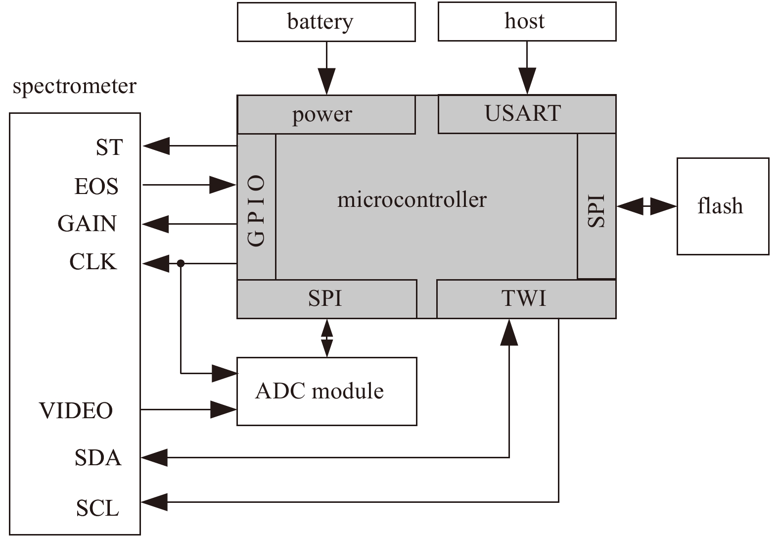
An 8-bit low-power microcontroller (ATxmega128A1U, Atmel Corporation, USA) is adopted to govern the operation of the spectrometer module and the relevant auxiliaries (Fig. 2). The primary motivation for choosing this chip is the abundance of onboard peripherals which greatly simply the design and integration of the various subsystems described below. The spectrometer prepares for the transmission of one group of spectral measurements upon receiving the rising edge at pin ST, and sequentially outputs each of the 256 voltage signals corresponding to the 256 photodiodes comprising the image sensor via pin VIDEO upon each rising edge of the pin CLK (Table 2). After the voltage signal for the last photodiode is sent, pin EOS of the spectrometer will be pulled low to indicate the completion of the data transmission. A 16-bit ADC (AD7988-5, Analog Devices Inc., USA) is used to digitize the analog output of the spectrometer. The reference voltage for the ADC is generated by an ultralow noise voltage reference chip (ADR435B, Analog Devices Inc., USA) with a nominal voltage of 5 V, which is wide enough to cover the entire output range of the spectrometer since the maximum output voltage of the spectrometer is approximately 4.4 V. To minimize temperature-induced biases in integration time of the spectrometer (i.e., the time interval between two adjacent ST pulses) over the entire operating temperature of –50°C to 30°C, a temperature compensated crystal oscillator (TCXO) is attached to the microcontroller to function as the system clock.
Figure
2.
Block diagram of the spectrometer and its driver electronics.
In addition, readout temperature of the spectrometer as indicated by an onboard 12-bit temperature sensor (DS1775R, Maxim Integrated Products, USA) is accomplished through a two-wire interface (TWI) of the microcontroller. Storage of spectral measurements to an external flash memory is realized via a serial peripheral interface (SPI), and one universal synchronous and asynchronous serial receiver and transmitter (USART) is reserved for system debugging. The entire system is powered by a 12 V battery pack, and peak power consumption is approximately 0.3 W when the spectrometer is in operation. To conserve power, sleep mode is activated during inactive times.
3.
Laboratory testing
As stated above, temperature is a vital concern when using a spectrometer in the cold polar environment, since temperatures in the Arctic winter (e.g., –40°C) are far below the minimum operating temperature of the spectrometer (i.e., 5°C) specified by the manufacturer. Further, this extremely low ambient temperature, is also very close to the minimum operating temperature of most electronic components. Temperature-induced mechanical distortion or stretching of the optical bench, or performance variation of the module’s electronics might alter the performance of the spectrometer. However, due to the limited availability of electrical power (i.e., battery pack), temperature stabilization of the spectrometer is not feasible during field deployment. Therefore, careful evaluation of the temperature and integration time dependence of the spectrometer are essential for use of any spectrometer in such cold environments, especially over seasonal time scales. It is noteworthy to mention that the output of the C11010MA spectrometer module is composed of two combined components of signal output and dark output. The former is generated by the incident light and determined by the intensity of the incident light and integration time. Whereas, the latter is the spectrometer output in the absence of any light and is composed of the dark voltage of the photodiode array and an offset voltage inherent to the internal charge amplifier. Thus, the characteristics of linear operating range, dark output, and signal output of the spectrometer are assessed in this study.
To quantify the temperature and integration time dependence of the spectrometer module, we placed it inside an environmental test chamber (GDS-500, Ayashilin, China) together with the relevant driver electronics, and made measurements under constant illumination, gradually lowering the temperature from 30°C to –50°C at an interval of 5°C (Fig. 3). This 80°C range of test temperatures should cover the annual temperature variation in the Arctic sea ice environment. A tungsten halogen bulb (6319, Newport Corporation, USA) was used as the light source. It was placed at room temperature (i.e., approximately 25°C) and was powered by a stabilized DC power supply, to ensure stability. The emitted light was split by a beam splitter, one beam was guided to the spectrometer via an optical fiber, the other beam was guided to a photodiode (DET100A/M, Thorlabs, Inc., USA) to monitor for intensity fluctuations of the light source during measurements. At each measurement temperature, we waited approximately 30 min for the spectrometer temperature to stabilize, as indicated by the onboard temperature sensor. We then measured spectrometer output over 15 different integration times ranging from 0.001 s to 16 s. The primary consideration for choosing such an integration time range is to make the spectrometer output fall in the linear and non-linear operating region for the shorter and longer integration time, respectively. The measurement was carried out 20 times for each integration time, to minimize the statistical uncertainty. Meanwhile, we also measured the dark output of the spectrometer at each of the above test temperatures for 17 integration time lengths ranging from 0.001 s to 30 s (including the 15 integration time lengths adopted above), by blocking the emitted light from entering the spectrometer via inserting an opaque board in the filter holder (Fig. 3).
Figure
3.
Configuration of the C11010MA spectrometer used to measure the spectrometer output and dark output.
Dark output is always a component of the spectrometer output regardless of the existence of incident light. From an application perspective (e.g., using the spectrometer to measure the incident light intensity), it should be removed from the spectrometer output to obtain the signal output only. To facilitate the correction of dark output, the temperature and integration time dependence of dark output were determined, and a prediction model was developed, based on the above measurement in the absence of any light signal.
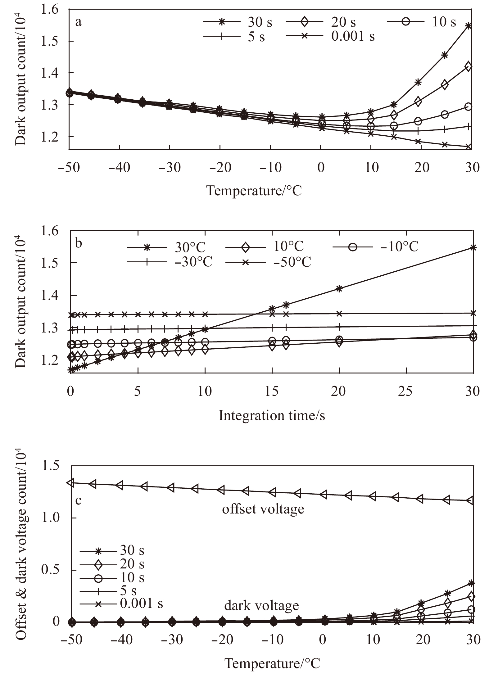
We observed that the dark output of the spectrometer varied considerably with temperature. It decreased roughly linearly with increasing temperature when it was below –10°C, and in the region below –10°C the dark output was almost independent of integration time (Fig. 4a). Above –10°C, the dark output was more dependent on integration time especially for those longer than 5 s. At each test temperature, we found that the relationship between dark output and integration time was strongly linear (Fig. 4b). The slope of the line increased and the intercept decreased as temperature increased. However, dark output was almost independent of integration time (constant) for temperatures below –10°C. These complicated characteristics are ascribed to the combined effects of an offset voltage and dark voltage.
Figure
4.
Dark output as a function of temperature at five integration times (a), and integration time at five test temperatures (b), and temperature dependence of offset voltage and dark voltage at five integration times (c).
Based on the preceding analysis, we determine that offset voltage arises from the internal charge amplifier which should be independent of integration time. Whereas, dark voltage derives from dark current within the surface and depletion layers of the photodiode, which should increase with longer integration times because more charge will be accumulated and integrated (Kuusk, 2011; Min et al., 2008). Since the offset voltage and dark voltage cannot be measured directly for this spectrometer module (the charge amplifier cannot be accessed directly), an analytical approach was adopted to separate the two components. At each test temperature, a linear model was applied to the relationship between dark output and integration time, and the fitted intercept was used to approximate the offset voltage. The difference between the dark output and the fitted offset voltage was used to approximate the dark voltage. The results demonstrated that the offset voltage decreased linearly with increasing temperature (Fig. 4c). Therefore, a linear model was adopted to represent offset voltage Voff as a function of temperature T by
where aoff and boff are the least squares fit intercept and slope, with the values of 12 290 counts and –21.29 counts/°C, respectively. The goodness of the linear fit as indicate by R2 is higher than 0.999 0.
For each integration time, the dark voltage was very close to 0 at temperatures below –10°C, but increased exponentially with increasing temperature for the higher temperature curves (Fig. 4c). Thus, an exponential model was used to parameterize the dark voltage Vdk as a function of temperature T for each integration time ti by
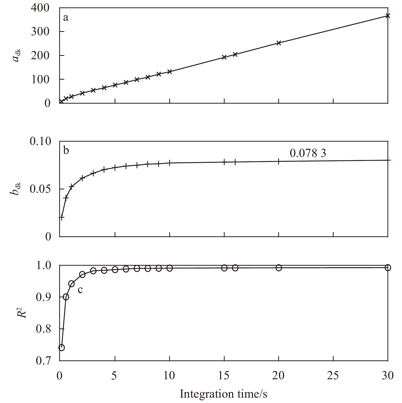
where adk(ti) and bdk(ti) are the least squares fit coefficients at ti. The fitted coefficient adk increased linearly with increased integration time for integration times longer than 0.1 s, and bdk was almost constant at 0.078 3 for integration times longer than approximately 5 s (Figs 5a and b). The goodness of the exponential fit indicated by R2 is higher than 0.9473 for integration times longer than 1 s (Fig. 5c). The uncertainty was relatively higher for the shorter integration times possibly because the corresponding dark voltage was very close to the noise level of the dark output. Thus, a linear model was adopted to approximate adk as a function of integration time t by
Figure
5.
Time dependence of the least squares fit coefficients adk (a) and bdk (b); the goodness of fit of Vdk (c) is shown for all integration times.
where $a_{\mathrm{dk}}'$ and $a_{\mathrm{dk}}''$ are the least squares fit coefficients with the values of 13.75 and 11.88, respectively. By replacing adk with Eq. (3) and setting bdk as a constant (i.e., 0.0783), Eq. (2) can be rewritten as
Summing this predicted dark voltage with the modeled offset voltage given by Eq. (1), the dark output of the spectrometer Vdark for any given t and T can be modeled as
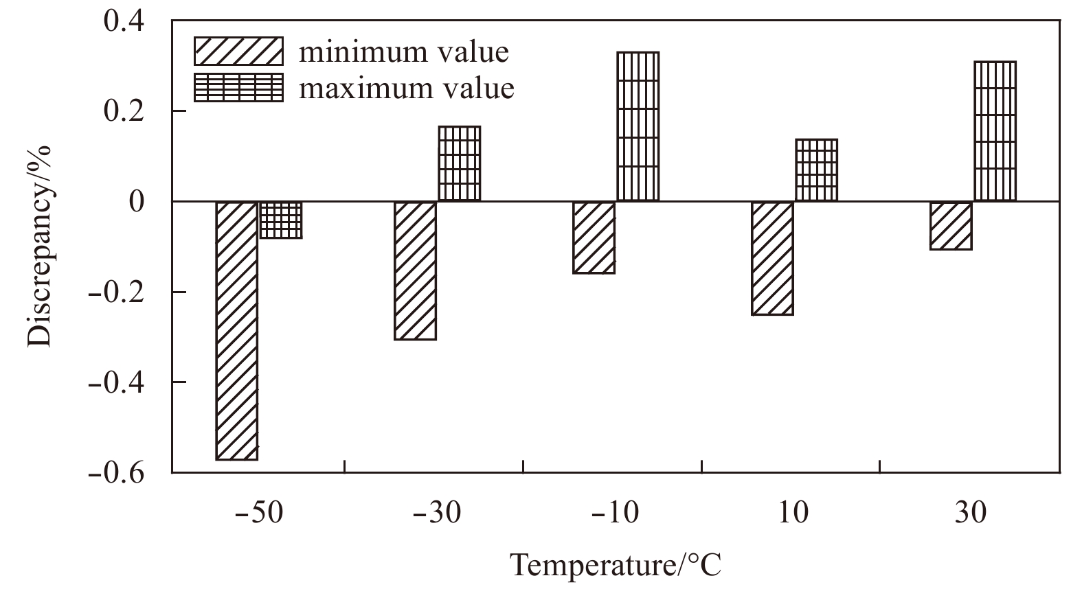
To evaluate the uncertainty of the dark output prediction model of Eq. (5), we independently measured dark output with a constant integration time of 5 s when temperature of the spectrometer decreased from 30°C to –50°C at 20°C interval. This temperature range was selected to validate the performance of the dark output prediction model over the entire 80°C range of operating temperatures of the spectrometer. The model predicted dark outputs agreed well with the measured values, on a pixel to pixel basis, with a maximum uncertainty of approximately ±0.6% for all the wavelengths considered (Fig. 6). The results indicate the prediction model can provide an accurate estimation of dark output in situations where dark output could not be measured directly or the system power consumption is a vital concern (e.g., for our application).
Figure
6.
The maximum and minimum values of the discrepancy between the modeled dark output and dark output derived from measurements for each of the five verification temperatures.
Making the spectrometer operate in the linear operating region is critical to accurately deriving the incident light intensity from the spectrometer output. The operating mechanism of the spectrometer is such that, any charges, no matter whether they are generated by the incident light or dark current are stored by the junction capacitance of the photodiode. As a result of the limited volume of the junction, the capacitance is limited, thus, the spectrometer operates linearly within some limit (i.e., the linear operating region), however, nonlinearity or saturation occur outside this limit (i.e., the nonlinear operating region). Because information about the linear operating region of the spectrometer module was unavailable, this was determined in this section using the above measurements under constant illumination.
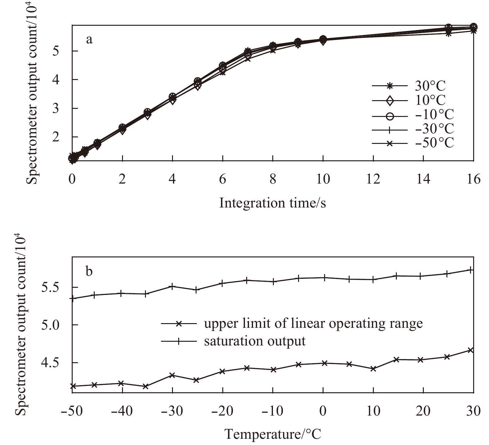
We first averaged the spectrometer output for each integration time over the times collected at each test temperature. We then picked out the maximum value of each averaged group of 256 spectrometer outputs (i.e., corresponding to pixel 49, wavelength 725 nm) and used them to analyze the linear operating region of the spectrometer. Spectrometer output was found to increase linearly with longer integration times for integration times below 7 s for the light source of this study (Fig. 7a). Between 7 s and 16 s, spectrometer output still increased with longer integration times, but the rate of increase gradually decreased. Above 16 s, spectrometer output was saturated and stable at a constant value. These characteristics were very similar for all test temperatures of –50°C to 30°C. The saturation output Vsat increased linearly with increasing temperature from 53 433 counts at –50°C to 57 312 counts at 30°C, and is approximated by
Figure
7.
Time dependence of the spectrometer output at five temperatures (a), and temperature dependence of the spectrometer saturation output and upper limit of the linear operating range (b).
where asat and bsat are the least squares fit coefficients with the values of 55 981 counts, and 42.16 counts/°C, respectively, and R2 is 0.915 5 (Fig. 7b).
Because the upper limit of the linear operating region of the spectrometer was not measured directly in this study, it was approximated analytically. At each test temperature, two lines were fitted to represent the spectrometer output as a function of integration time, with one using the measurements within the linear operating region (i.e., integration time ≤7 s) and the other using the two measurements adjacent to the linear operating region (i.e., integration time was 8 s and 9 s). The vertical coordinate value of the two lines was used to approximate the upper limit of the linear operating region Vul. We observed that the approximated Vul also increased linearly with increasing temperature from 41 858 counts at –50°C to 46 669 counts at 30°C, as expressed by
where aul and bul are the least squares fit coefficients, with values of 44 583 counts, and 55.53 counts/°C, respectively, and R2 is 0.913 6 (Fig. 7b). It should be emphasized that the temperature dependence of Vul is a superposition of the dark output and signal output. When the dark output given by Eq. (5) was subtracted from Vul given by Eq. (7), the complete linear operating region of the spectrometer Vlor could be inferred and is given by
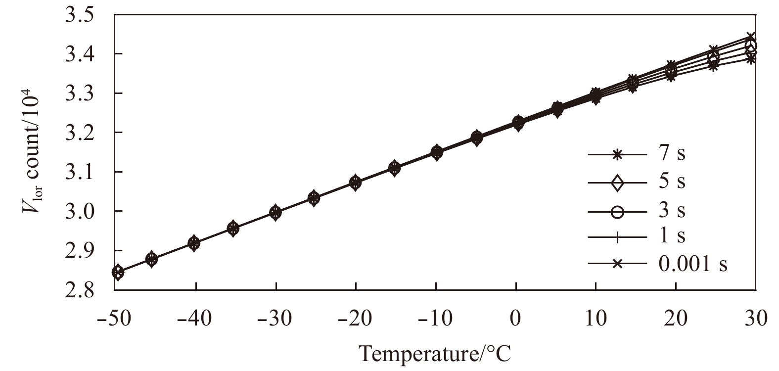
It is determined that Vlor increased with increasing temperature over the entire operating temperature range of –50°C to 30°C, with an increment of approximately 17.4% at 1 s from –50°C to 30°C (Fig. 8). This relationship was linear and not sensitive to integration time at temperatures below 5°C. However, above 5°C, the influence of integration time on Vlor was more significant for the warmer temperatures and longer integration times, because the influence of dark voltage was more significant under these circumstances.
Figure
8.
Temperature dependence of the linear operating region of the spectrometer at five integration times.
4.3.1
Temperature and integration time dependence of signal output
Signal output is excited by the incident light, therefore, detailed information about how signal output changes with temperature and integration time is essential to accurately quantify the incident light intensity based on the signal output collected at varied temperature and integration times during field application. Using the spectral measurements collected under the constant illumination in Section 3, we first subtracted the dark output from the spectrometer output to obtain the signal output. We then averaged the signal output over the times collected for each integration time at each temperature, to minimize the influence of statistical uncertainty during the examination. We finally corrected the influence of light source fluctuations in the averaged signal output as indicated by the photodiode, by referencing the corresponding photodiode voltage to that of the first measurement (i.e., integration time 0.001 s and temperature 30°C).
The results indicate that the general shape of the signal output, which was primarily determined by the spectral sensitivity of the spectrometer and the spectral shape of the incident light source, is very similar for each integration time over the entire 80°C range of operating temperatures (Fig. 9a). Signal output generally decreased with lower temperatures approximately parabolically for each wavelength, more significantly for longer wavelengths, with a magnitude of around 45.2% from 30 to –50°C at 1 000 nm (Figs 9a and b). However, signal output increased linearly with longer integration times when the spectrometer operated in the linear operating region (the integration time is shorter than 7 s for the light source adopted in this study; Fig. 9c). This characteristic verified that the C11010MA miniature spectrometer can operate stably and reliably even at temperatures far below the minimum operating temperature specified by the vendor, and is appropriate for our application.
Figure
9.
Signal output as a function of wavelength for five test temperatures at 1 s integration time (a), temperature for five wavelengths at 1 s integration time (b), and integration times for five wavelengths at –50°C (c). Marker styles in (b) and (c) are the same.
4.3.2
Development of signal output correction models
In Section 4.3.1, temperature and integration time dependence of the spectrometer signal output were evaluated performing measurements under a tungsten halogen bulb. Based on the results, signal output correction models, which can be used to correct the temperature-induced biases in the signal output under incident light sources besides the light bulb adopted in this study, can be developed. Assuming the temperature and integration time dependence of the spectrometer are stable and independent of light source, signal correction models are investigated in this section to convert the signal output measured at any temperature and integration time to the value that would be measured at a reference temperature and reference integration time, Tref and tref, respectively. Tref and tref were selected as 25°C and 1 s.
To accomplish this, we first calculated the relative change in signal output (i.e., relative signal output) by referencing the corrected signal outputs (i.e., those in Section 4.3.1) to those taken at Tref and tref. It could be inferred that temperature and integration time dependence of the relative signal output were very similar to that of the signal output. In other words, the temperature dependence of the relative signal output was approximately parabolic, and the integration time dependence of the relative signal output was linear, for each wavelength (Fig. 10). We developed two different signal output correction models (namely, Model I and Model II), to be discussed in the following, based on temperature and integration time dependence of the relative signal output.
Figure
10.
The relative signal output as a function of temperature at 1 s integration time (a), and integration time at –50°C (b) for five wavelengths.
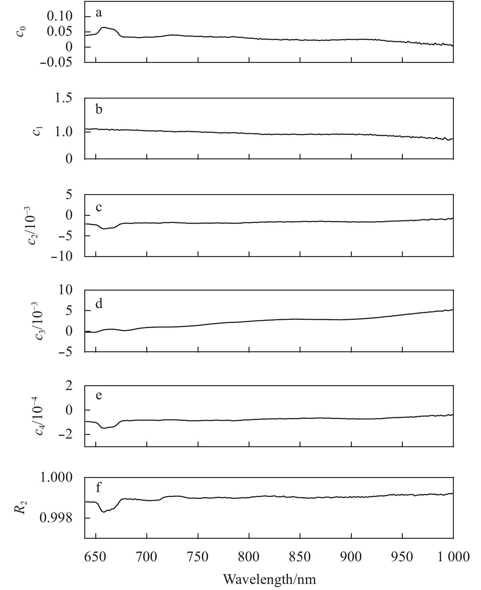
For Model I, a polynomial was used to approximate the relative signal output f as a function of temperature T and integration time t as
$$
f(\lambda, t, T)= c_{0}(\lambda)+c_{1}(\lambda) t+c_{2}(\lambda) T +c_{3}(\lambda) t T+c_{4}(\lambda) T^{2},
$$
(9)
where c0 to c4 are the least squares fit coefficients at each wavelength λ (Figs 11a-e). The goodness of fit of f as indicated by R2 is higher than 0.998 3 for all wavelengths (Fig. 11f).
Figure
11.
The least squares fit coefficient c0–c4 (a–e), and the goodness of the fit to f (f) as a function of wavelength.
where d0 and d1 are the least squares fit coefficients at each wavelength λ and temperature T (Figs 12a and b), and R2 is higher than 0.999 8 for all wavelengths (Fig. 12c). We observed that the fitted intercept d0 was relatively stable with temperature over the entire 80°C range of operating temperatures, and the fitted slope d1 generally decreased at lower temperatures in an approximately parabolic manner. As a result, a linear model, and a second order polynomial model were adopted to represent d0, and d1, respectively, as a function of temperature by
Figure
12.
The least squares fit coefficient d0 (a), and d1 (b) as a function of temperature at five wavelengths; the goodness of fit to f (c) as a function of wavelength at five temperatures.
where d00, d01, and d10 to d12 are the least squares fit coefficients. By replaying d0 and d1 with Eqs (11) and (12), Eq. (10) could be rewritten as
$$
f(\lambda, t, T)= d_{00}(\lambda)+d_{01}(\lambda) T +\left[d_{10}(\lambda)+d_{11}(\lambda) T+d_{12}(\lambda) T^{2}\right] t.
$$
(13)
4.3.3
Verification of signal output correction models
To assess the practicality and uncertainty of the signal output correction models developed above, we employed an experimental setup similar to that shown in Fig. 3, apart from the addition of a neutral density filter with a nominal transmittance of 79% inserted between the lens and beam splitter to change the intensity of the light entering the spectrometer. We measured the spectrometer output with a constant integration time of 1 s at three operating temperatures of 30°C, –10°C, and –50°C. At each temperature, as before, we waited around 30 minutes for the temperature of the spectrometer module to stabilize before collecting measurements, which were then conducted 20 times to minimize statistical uncertainty. The dark output of the spectrometer for each temperature was also measured for the subsequent correction. Spectrometer output and dark output at Tref (i.e., 25°C) and tref (i.e., 1 s) were also measured.
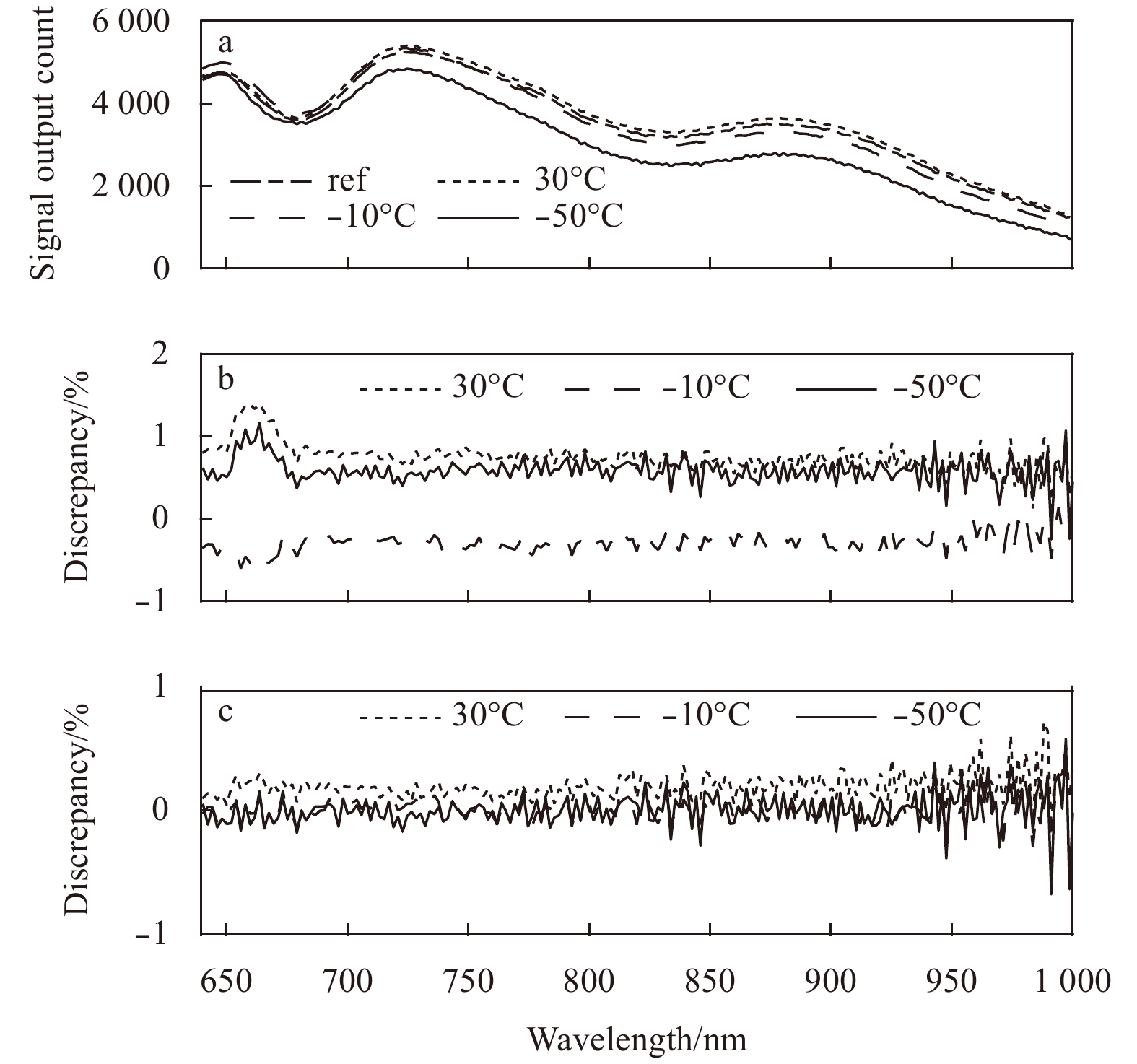
To analyze the data, we first subtracted the dark output from the spectrometer output to obtain the signal output. We next averaged the signal output over the measurements collected and corrected the influence of light source fluctuation. The results indicated that signal output generally decreased at lower temperatures, with a reduction of approximate 45.4% at 1 000 nm when the temperature decreased from 30°C to –50°C (Fig. 13a). These temperature-induced biases in the signal output agreed well with those obtained in Section 3 (without a neutral density filter), verifying that the temperature dependence of the spectrometer is stable and independent of light source intensity to a certain degree. We corrected the signal outputs using Model I and Model II and the fitted coefficients (Eqs (9) and (13), respectively), to convert measurements made at three temperatures to measurements corresponding to measurements made at Tref and tref. Compared with the signal output measured directly at Tref and tref, we found that the uncertainty of Model I was within ±1.5% over the entire wavelength range of 640–1 000 nm (Fig. 13b). Whereas, the uncertainty of Model II was even better than that of Model I, with a value of approximately ±0.5% for wavelengths shorter than 980 nm (Fig. 13c). From the perspective of minimizing the temperature-induced biases in the signal output as much as possible, Model II was preferred and adopted in this study.
Figure
13.
Signal output as a function of wavelength at the reference temperature together with three verification temperatures (a), and discrepancy of Model I (b) and Model II (c) as a function of wavelength at three verification temperatures.
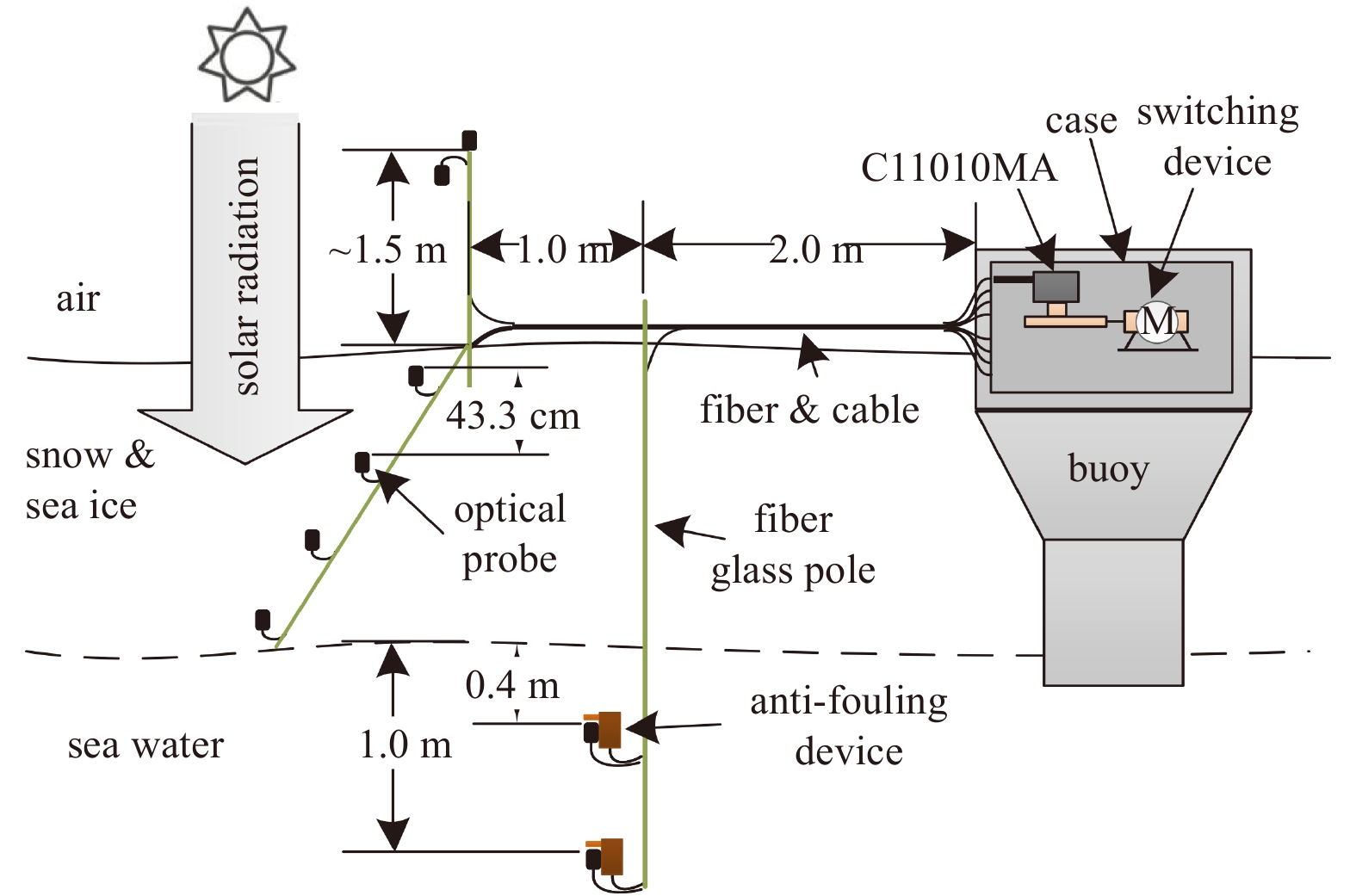
To testify the overall performance of the C11010MA miniature spectrometer module, it was integrated into a refined fiber optic spectrometry system together with the relevant driver electronics and measured the solar irradiance distribution within the ice cover with an ice thickness of 1.75 m and snow thickness of 0.1 m during the 9th Chinese National Arctic Research Expedition. The solar radiation signals at 8 different levels of the sea ice were collected and transmitted by 8 fiber probes included in the spectrometry system, respectively. The distribution of the fiber probes was shown in Fig. 14. Two probes were placed ~1.5 m above the snow surface to measure the downwelling and upwelling solar irradiance signals separately. Four probes were embedded within the ice cover at a vertical depth interval of 0.434 m, with the upmost probe located at a distance of 0.1 m below the snow surface. The remaining two probes were deployed 0.4 and 1 m below the ice bottom, respectively. The spectrometer was aligned to each of the fiber probe in sequence under the control of a rotary spectrometer switching device. Spectral sensitivity of each combination of the spectrometer and each of the fiber probe was determined by a simultaneous comparison study carried out using a radiometrically calibrated hyperspectral irradiance sensor (RAMSES-ACC-VIS, TriOS Mess- und Datentechnik GmbH, Germany) as a standard, at room temperature (i.e., 25°C).
Figure
14.
Deployment scenario of the irradiance profiling system where the main body.
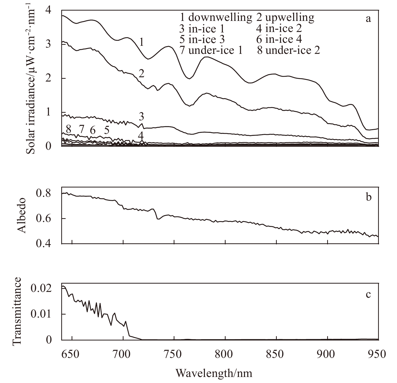
To determine solar irradiance at different levels of the sea ice environment, we first corrected the influence of dark output in the spectral measurement by subtraction to get the signal output. The dark output was estimated using Eq. (5) with the same integration time as the corresponding spectral measurement and temperature of the spectrometer module as the inputs. We then converted the signal output to that at Tref and tref by dividing with Eq. (13). We finally corrected spectral sensitivity of the spectrometer and fiber probe to get spectral intensity of the solar irradiance. The results denoted that general shape of the solar irradiance at different level of the sea ice was similar, and general shape of the solar irradiance above the snow surface measured by the spectrometer agreed well with that measured by other oceanographic spectroradiometers (Fig. 15a) (Nicolaus et al., 2010). However, spectral intensity of the solar irradiance decreased much faster at the near-infrared region than at the visible region, as the position is deeper in the ice (lines 3–6 in Fig. 15a) and in the underlying water (lines 7 and 8 in Fig. 15a). This characteristic ascribed to the fact that spectral absorption coefficient of the ice and water was much bigger at the near-infrared region than at the visible region (Grenfell and Perovich, 1981). When we calculated the spectral albedo of the sea ice using the upwelling irradiance to divide the downwelling irradiance above the snow surface (i.e., lines 1 and 2 in Fig. 15a), we found that spectral albedo of the sea ice generally decreased with longer wavelengths, from 0.80 at 640 nm to 0.46 at 950 nm (Fig. 15b). This characteristic basically agreed with spectral albedo of the sea ice covered with melting old snow (Riihelä et al., 2013). Spectral transmittance of the sea ice (i.e., 1.75 m sea ice covered with 0.1 m snow) was also calculated by using the downwelling irradiance below the ice bottom (line 7 in Fig. 15a) to divide that above the snow surface (line 1 in Fig. 15a). It indicated that spectral transmittance of the sea ice generally decreased with longer wavelengths with the biggest value of 0.021 at 640 nm. The transmittance was very close to 0 for wavelengths longer than 710 nm because there is almost no light within these bands transmitted through the sea ice and detected by the spectrometer (Fig. 15c).
Figure
15.
Solar irradiance as a function of wavelength at different levels of the sea ice environment (a), and spectral albedo (b) and spectral transmittance (c) as a function of wavelength for the sea ice the spectrometer deployed.
In this study, the feasibility of employing a miniature near-infrared spectrometer in a cold sea ice environment has been assessed and verified. The temperature dependence and integration time dependence of the spectrometer output and dark output have been measured over the entire operating temperature range of –50°C to 30°C, well below the stated operating range of this spectrometer. The results indicate that the offset voltage decreases linearly with increasing temperature and dark voltage increases exponentially with increasing temperatures at temperatures above –10°C. A dark output prediction model is developed to represent the dark output as a function of temperature and integration time with an uncertainty of ±0.6% for all wavelengths of interest. The saturation output and upper limit of the linear operating region of the spectrometer increase with increasing temperature, at a rate of 42.16 counts/°C and 55.53 counts/°C, respectively. Signal output increases with increasing temperature in an approximately parabolic manner when the spectrometer is operated in the linear operating range. However, it increases linearly with longer integration times over the entire operating temperature of –50°C to 30°C. Two signal output correction models are developed and compared to convert the signal output measured at any temperature within the operating range and integration time to that measured at the reference temperature Tref and integration time tref, with respective model uncertainties of ±1.5% and ±0.5% for the spectral range considered. The overall performance of the spectrometer module is testified in an ice pack in the Arctic. The results denote that the general shape of the solar irradiance above the snow surface measured by the spectrometer agrees well with that at the sea level, as measured by other commercially available oceanographic spectroradiometers. Additionally, the calculated optical properties of the sea ice where the spectrometer is deployed are identical to those pertaining to similar sea ice calculated from measurements by other researches. Power consumption of the spectrometer together with its driver electronics is ~265 mW in working mode and ~10 mW in idle mode in its current configuration. Given that the spectrometer makes measurement once a day with the measurement time of 15 min, a battery with a capacity of at least 9 800 mAh is needed to maintain the normal operation of spectrometer for 12 months. Future work will focus on longer-term change assessment in stability or sensitivity of the spectrometer, field verification of the spectrometer performance, and comparative measurements between this spectrometer and oceanographic spectrometers to further determine the feasibility of the spectrometer.
Campbell K, Mundy C J, Barber D G, et al. 2015. Characterizing the sea ice algae chlorophyll a–snow depth relationship over Arctic spring melt using transmitted irradiance. Journal of Marine Systems, 147: 76–84. doi: 10.1016/j.jmarsys.2014.01.008
[2]
Comiso J C, Parkinson C L, Gersten R, et al. 2008. Accelerated decline in the Arctic sea ice cover. Geophysical Research Letters, 35(1): L01703
[3]
Ehn J K, Papakyriakou T N, Barber D G. 2008. Inference of optical properties from radiation profiles within melting landfast sea ice. Journal of Geophysical Research: Oceans, 113(C9): C09024
[4]
Ehn J K, Mundy C J, Barber D G, et al. 2011. Impact of horizontal spreading on light propagation in melt pond covered seasonal sea ice in the Canadian Arctic. Journal of Geophysical Research: Oceans, 116(C9): C00G02
[5]
Feister U, Grewe R. 1995. Spectral albedo measurements in the UV and visible region over different types of surfaces. Photochemistry and Photobiology, 62(4): 736–744. doi: 10.1111/j.1751-1097.1995.tb08723.x
[6]
Frey K E, Perovich D K, Light B. 2011. The spatial distribution of solar radiation under a melting Arctic sea ice cover. Geophysical Research Letters, 38(22): L22501
[7]
Grenfell T C, Light B, Perovich D K. 2006. Spectral transmission and implications for the partitioning of shortwave radiation in arctic sea ice. Annals of Glaciology, 44: 1–6
[8]
Grenfell T C, Perovich D K. 1981. Radiation absorption coefficients of polycrystalline ice from 400–1400 nm. Journal of geophysical research, 86(C8): 7447-7450
[9]
Kuusk J. 2011. Dark signal temperature dependence correction method for miniature spectrometer modules. Journal of Sensors, 2011: Article ID 608157
[10]
Lei Ruibo, Leppäranta M, Erm A, et al. 2011. Field investigations of apparent optical properties of ice cover in Finnish and Estonian lakes in winter 2009. Estonian Journal of Earth Sciences, 60(1): 50. doi: 10.3176/earth.2011.1.05
[11]
Lei Ruibo, Zhang Zhanhai, Matero I, et al. 2012. Reflection and transmission of irradiance by snow and sea ice in the central Arctic Ocean in summer 2010. Polar Research, 31(1): 17325. doi: 10.3402/polar.v31i0.17325
[12]
Light B, Grenfell T C, Perovich D K. 2008. Transmission and absorption of solar radiation by Arctic sea ice during the melt season. Journal of Geophysical Research: Oceans, 113(C3): 03023. doi: 10.1029/2006JC003977
[13]
Maslanik J A, Fowler C, Stroeve J, et al. 2007. A younger, thinner Arctic ice cover: Increased potential for rapid, extensive sea-ice loss. Geophysical Research Letters, 34(24): L24501. doi: 10.1029/2007GL032043
[14]
Maslanik J, Stroeve J, Fowler C, et al. 2011. Distribution and trends in Arctic sea ice age through spring 2011. Geophysical Research Letters, 38(13): L13502
[15]
Min M, Lee W S, Burks T F, et al. 2008. Design of a hyperspectral nitrogen sensing system for orange leaves. Computers and Electronics in Agriculture, 63(2): 215–226. doi: 10.1016/j.compag.2008.03.004
[16]
Nicolaus M, Hudson S R, Gerland S, et al. 2010. A modern concept for autonomous and continuous measurements of spectral albedo and transmittance of sea ice. Cold Regions Science and Technology, 62(1): 14–28. doi: 10.1016/j.coldregions.2010.03.001
[17]
Nicolaus M, Katlein C. 2013. Mapping radiation transfer through sea ice using a remotely operated vehicle (ROV). The Cryosphere, 7(3): 763–777. doi: 10.5194/tc-7-763-2013
[18]
Palmer M A, Saenz B T, Arrigo K R. 2014. Impacts of sea ice retreat, thinning, and melt-pond proliferation on the summer phytoplankton bloom in the Chukchi Sea, Arctic Ocean. Deep Sea Research Part Ⅱ: Topical Studies in Oceanography, 105: 85–104. doi: 10.1016/j.dsr2.2014.03.016
[19]
Perovich D K, Grenfell T C, Light B, et al. 2002. Seasonal evolution of the albedo of multiyear Arctic sea ice. Journal of Geophysical Research: Oceans, 107(C10): SHE 20-1–SHE 20-13
[20]
Perovich D K, Jones K F, Light B, et al. 2011. Solar partitioning in a changing Arctic sea-ice cover. Annals of Glaciology, 52(57): 192–196. doi: 10.3189/172756411795931543
[21]
Pirazzini R, Vihma T, Granskog M A, et al. 2006. Surface albedo measurements over sea ice in the Baltic Sea during the spring snowmelt period. Annals of Glaciology, 44: 7–14. doi: 10.3189/172756406781811565
[22]
Riihelä A, Manninen T, Laine V. 2013. Observed changes in the albedo of the Arctic sea-ice zone for the period 1982–2009. Nature Climate Change, 3(10): 895–898. doi: 10.1038/nclimate1963
[23]
Serreze M C, Holland M M, Stroeve J. 2007. Perspectives on the Arctic's shrinking sea-ice cover. Science, 315(5818): 1533–1536. doi: 10.1126/science.1139426
[24]
Stroeve J C, Serreze M C, Holland M M, et al. 2012. The Arctic’s rapidly shrinking sea ice cover: a research synthesis. Climatic Change, 110(3–4): 1005–1027
[25]
Treffeisen R, Krejci R, Ström J, et al. 2007. Humidity observations in the Arctic troposphere over Ny-Ålesund, Svalbard based on 15 years of radiosonde data. Atmospheric Chemistry and Physics, 7(10): 2721–2732. doi: 10.5194/acp-7-2721-2007
[26]
Wang Hangzhou, Chen Ying, Song Hong, et al. 2014. A fiber optic spectrometry system for measuring irradiance distributions in sea ice environments. Journal of Atmospheric and Oceanic Technology, 31(12): 2844–2857. doi: 10.1175/JTECH-D-14-00108.1
Liwen Nan, Xiaoping Wang, Hangzhou Wang, Hongliang Zhou, Ying Chen. Feasibility study of miniature near-infrared spectrometer for the measurement of solar irradiance within Arctic snow-cover sea ice[J]. Acta Oceanologica Sinica, 2020, 39(9): 115-124. doi: 10.1007/s13131-020-1632-y
Liwen Nan, Xiaoping Wang, Hangzhou Wang, Hongliang Zhou, Ying Chen. Feasibility study of miniature near-infrared spectrometer for the measurement of solar irradiance within Arctic snow-cover sea ice[J]. Acta Oceanologica Sinica, 2020, 39(9): 115-124. doi: 10.1007/s13131-020-1632-y
Figure 1. Schematic diagram of the C11010MA miniature spectrometer.
Figure 2. Block diagram of the spectrometer and its driver electronics.
Figure 3. Configuration of the C11010MA spectrometer used to measure the spectrometer output and dark output.
Figure 4. Dark output as a function of temperature at five integration times (a), and integration time at five test temperatures (b), and temperature dependence of offset voltage and dark voltage at five integration times (c).
Figure 5. Time dependence of the least squares fit coefficients adk (a) and bdk (b); the goodness of fit of Vdk (c) is shown for all integration times.
Figure 6. The maximum and minimum values of the discrepancy between the modeled dark output and dark output derived from measurements for each of the five verification temperatures.
Figure 7. Time dependence of the spectrometer output at five temperatures (a), and temperature dependence of the spectrometer saturation output and upper limit of the linear operating range (b).
Figure 8. Temperature dependence of the linear operating region of the spectrometer at five integration times.
Figure 9. Signal output as a function of wavelength for five test temperatures at 1 s integration time (a), temperature for five wavelengths at 1 s integration time (b), and integration times for five wavelengths at –50°C (c). Marker styles in (b) and (c) are the same.
Figure 10. The relative signal output as a function of temperature at 1 s integration time (a), and integration time at –50°C (b) for five wavelengths.
Figure 11. The least squares fit coefficient c0–c4 (a–e), and the goodness of the fit to f (f) as a function of wavelength.
Figure 12. The least squares fit coefficient d0 (a), and d1 (b) as a function of temperature at five wavelengths; the goodness of fit to f (c) as a function of wavelength at five temperatures.
Figure 13. Signal output as a function of wavelength at the reference temperature together with three verification temperatures (a), and discrepancy of Model I (b) and Model II (c) as a function of wavelength at three verification temperatures.
Figure 14. Deployment scenario of the irradiance profiling system where the main body.
Figure 15. Solar irradiance as a function of wavelength at different levels of the sea ice environment (a), and spectral albedo (b) and spectral transmittance (c) as a function of wavelength for the sea ice the spectrometer deployed.


 DownLoad:

 DownLoad:


 DownLoad: