Key Laboratory of Marine Geology and Environment, Institute of Oceanology, Chinese Academy of Sciences, Qingdao 266071, China
2.
Laboratory for Marine Geology, Pilot National Laboratory for Marine Science and Technology (Qingdao), Qingdao 266237, China
3.
Center for Ocean Mega-Science, Chinese Academy of Sciences, Qingdao 266071, China
4.
University of Chinese Academy of Sciences, Beijing 100049, China
Funds:
The National Natural Science Foundation of China under contract Nos 41406215 and 41706194; a fund provided by the Qingdao National Laboratory for Marine Science and Technology; the National Natural Science Foundation of China (NSFC)-Shandong Joint Fund for Marine Science Research Centers under contract No. U1606401.
The spatial structure of the Arctic sea ice concentration (SIC) variability and the connection to atmospheric as well as radiative forcing during winter and summer for the 1979–2017 period are investigated. The interannual variability with different spatial characteristics of SIC in summer and winter is extracted using the empirical orthogonal function (EOF) analysis. The present study confirms that the atmospheric circulation has a strong influence on the SIC through both dynamic and thermodynamic processes, as the heat flux anomalies in summer are radiatively forced while those in winter contain both radiative and “circulation-induced” components. Thus, atmospheric fluctuations have an explicit and extensive influence to the SIC through complex mechanisms during both seasons. Moreover, analysis of a variety of atmospheric variables indicates that the primary mechanism about specific regional SIC patterns in Arctic marginal seas are different with special characteristics.
Additionally, there are studies examining the local correspondence between the atmospheric forcing and sea ice variability. Germe et al. (2011) found that the sea ice in the Greenland Sea is largely consistent with the wind anomalies as well as the surface air temperature (SAT) anomalies. Herbaut et al. (2015) suggested that surface winds explain approximately 50% of the SIC variance in the Barents Sea, while the residual is caused by the heat inflow related to Atlantic Water input. In addition, Nakanowatari et al. (2015) demonstrated that approximately 29% of the ice area variability in the Bering Sea is associated with changes in the geopotential height at 500 hPa (Z500) during the leading three-month period. Lynch et al. (2016) identified that the sectoral asymmetric sea ice anomalies in the Arctic are partly attributable to the atmospheric circulation in summer. These studies demonstrate both the large-scale and regional behaviors of the atmospheric forcing can impact the spatiotemporal variability in sea ice within the Arctic Ocean.
During the past two decades (1998–2018), the spatial and temporal characteristics of sea ice variability have changed significantly (Eisen and Kottmeier, 2000; Pleijter, 2014). For instance, Arctic Sea ice is decreasing in extent at an accelerated rate (Comiso et al., 2008), becoming thinner (Maslanik et al., 2007; Lindsay and Schweiger, 2015) due to a warmer climate, and transforming toward a younger ice pack (Maslanik et al., 2007, 2011). In addition, the enhanced SIC trend in the Barents Sea and Greenland Sea has recently become dominant (Deser and Teng, 2008; Pleijter, 2014), which leads to a potential shift in the variability structure of the winter SIC. However, the knowledge of the quantitative role of the varying forcing in the recent Arctic sea ice changes remains vague.
Based on satellite-derived SIC data over the 1979–2017 period, the aim of the present study is to investigate the two leading principal mode structures of SIC variability in the Arctic Ocean during both winter and summer seasons. The association with the distinct SIC variability due to different variables related to atmospheric forcings, including SAT and sea level pressure (SLP), are examined. Contrast to previous studies, here we draw attention on the second mode of interannual variations of SIC in two seasons, which were not discussed in details. Moreover, the regional SIC variability together with the relevant dynamic and thermodynamic mechanisms are outlined.
The paper is organized as follows. Datasets and analysis methods are described in Section 2. In Section 3, the retrieved EOF modes of SIC variability are presented. The relationship between the distinct mode of SIC variability and a variety of atmospheric variables (SAT, SLP and surface radiation, etc.) are analyzed in Section 4. The conclusions of this study are presented in Section 5.
2.
Data and methods
2.1
Data
Monthly SIC and Sea ice motion (SIM) data were obtained from the National Snow and Ice Data Center (NSIDC). SIC is derived from brightness temperature measured with a series of satellite-based radiometers by applying the Bootstrap algorithm (Comiso, 2017). It is available on a polar stereographic projection with a grid size of 25 km × 25 km. SIM fields are retrieved from multiple sources, including satellite measurements and buoy observations, as well as surface winds from the National Centers for Environmental Prediction and the National Center for Atmospheric Research (NCEP/NCAR). The SIM vectors has a grid cell size of 25 km × 25 km. The large-scale atmospheric index, AO (Thompson and Wallace, 1998), is provided by the NOAA Climate Prediction Center(CPC). Cryosphere Science Research Portal of NASA provides data of early melt (earliest observed melt conditions) and early freeze (earliest observed freeze conditions) for the surface of sea ice, the results are derived from SSM/I data following Markus et al. (2009) and use the same grid with SIC. Other variables including SLP, SAT, surface albedo, vertical integral of heat, water vapor flux, total column water vapor, total column water vapor, total cloud cover, surface net downward shortwave flux and surface net downward longwave flux are provided in a 2.5°×2.5° global grid, retrieved from ERA-Interim Archive at European Centre for Medium Range Weather Forecasts (ECMWF).
The seasonal division, appropriate for middle and high latitudes, could capture a better activity center if the atmospheric field is utilized (Fan et al., 2012). For all these data, the monthly means are used to extract the seasonal means for winter (December–March) and summer (June–September). The seasonal averages of all datasets for each year during 1979–2017 are calculated, and the anomaly field for each individual year is calculated by subtracting the 39-year climatology.
2.2
Methodology
The empirical orthogonal function (EOF) analysis was applied to retrieve the distinct mode of sea ice variability in different seasons, which accounts for a major fraction of the variance in SIC anomalies. This technique has been widely adopted because of its capacity to simultaneously obtain the temporal and spatial variabilities. The extracted spatial structure corresponds to a specific distribution pattern of SIC variations. The principal component (PC) time series of each mode is determined by projecting the derived orthogonal patterns onto the spatially weighted anomalies, and the PC represents a measure of the degree of similarity between the dominant pattern and an individual anomaly pattern.
Regression and correlation analyses are further used to assess the relationship between the variations in SIC and different variables. A regression analysis is applied on each grid to inspect the coupled mechanism between the atmospheric forcing and the PC time series of the SIC anomaly fields. A correlation analysis is used to examine the connection between two patterns or driving factors. We analyze interannual variability rather than the low-frequency changes which can confound the identification of physical mechanisms in the short period (1979 to present) for which high-quality sea ice data are available. Thus, prior to carrying out the regression and correlation analyses, the significant SIC trends are removed to characterize the interannual variations (King et al., 2016).
3.
Results
3.1
Spatiotemporal characteristics of SIC variability
3.1.1
Spatial structures and temporal changes in winter
Figure
1.
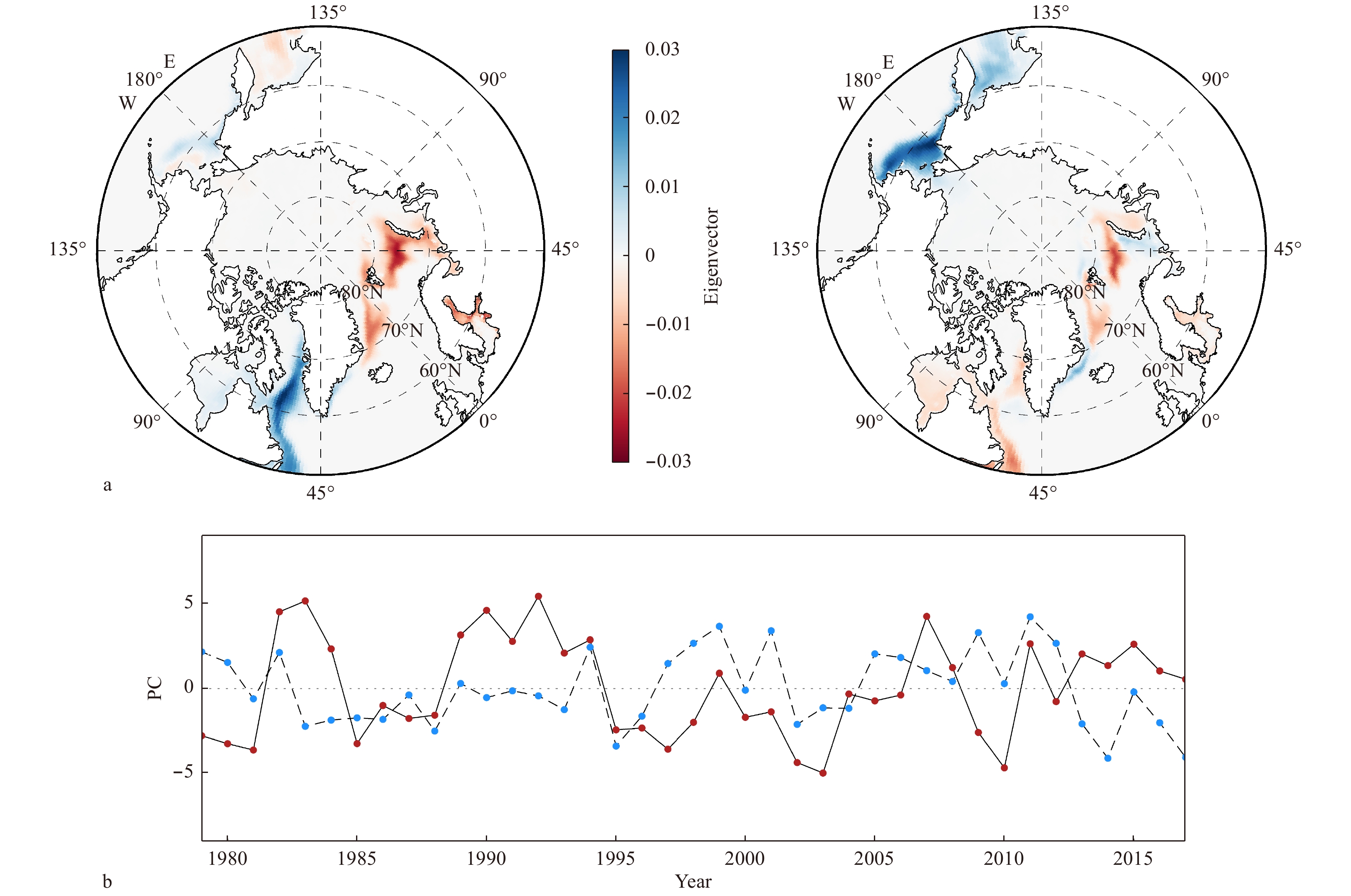
The first and second modes of SIC interannual variability in winter (December–March) in the Arctic Ocean over the period of 1979/1980–2017/2018 (a), and the associated PC time series (b). The solid line with red dots denotes the PC time series of the leading mode of EOF analysis and the dashed line with blue dots corresponds to the second mode. Note that the EOF analysis is applied over the SSM/I polar spatial coverage. The PC is normalized to the unit variance.
Based on the detrended SIC data, the first and second EOFs account for less variance than that based on raw data, approximately 21.4% and 11.9% (Table A1 in Appendix), respectively. The spatial pattern of the dominate mode exhibits out-of-phase variations between the Sea of Okhotsk, Bering Sea and between the Barents Sea as well as Labrador Sea (Fig. 1). The EOF1 pattern is largely consistent with the modes presented in previous studies (Fang and Wallace, 1994; Deser et al., 2000; Ukita et al., 2007). The second mode is characterized by a variability structure with roughly opposite sign located at around the Baffin Bay, Nordic seas and the Bering Sea, Sea of Okhotsk, respectively.
A1.
Percent variance explained by EOFs during 1979–2017
Interestingly, the leading EOF pattern is reminiscent of the wintertime trend pattern, with a high correlation coefficient of 0.978 (Fig. A1 in Appendix). Also, we identify that the second and third EOF mode, based on the original SIC data, correspond well to the first and second modes applied on detrended SIC data (with correlation coefficients of 0.91 and 0.92). These facts seem to suggest that the leading EOF mode using the raw data mostly captures the changes due to the linear trend in SIC, while the second EOF mode largely reflects a pattern associated with some interannual fluctuations. Owing to the strong negative trend in the SIC during winter in the past decades, the proportion of variability caused by the trend has become more significant and dominates the overall variability.
A1.
SIC trends in the Arctic Ocean in winter (1979/1980–2017/2018) (a), the first and second modes of SIC variability in winter (December–March) in the Arctic Ocean over the period of 1979/1980–2017/2018 based on raw data (b), and the associated PC time series (c). The solid line with red dots denotes the PC time series of the leading EOF analysis mode, and the dashed line with blue dots corresponds to the second mode. Black solid lines denote the trend that is significant at the 95% confidence level. Note that the EOF analysis is applied over the SSM/I polar spatial coverage.
3.1.2
Spatial structures and temporal changes in summer
Figure 2 shows the SIC anomaly EOF modes in summer (June–September). The leading mode explains 15.2% (Table A1 in Appendix) of the variance and is characterized by broad in-phase variability over the broad marginal seas from the Beaufort Sea eastward throughout the Kara Sea with a small contrary area northeastern of Greenland (Fig. 2a). According to the definition, a positive (negative) leading EOF index indicates a decline (an increase) in most marginal areas of the Arctic. In particular, the two outstanding positive values appearing in 2007 and 2012 are in tune with the two extreme minimums of the September SIE in the Arctic. Figure 2b reveal the second mode of SIC in summer, which shows a tri-pole feature in the Arctic marginal seas, with a decrease in the sea-ice variability mainly in the Chukchi Sea, East Siberian Sea and Laptev Sea, whereas the Beaufort Sea, Barents Sea and Kara Sea show the opposite pattern. The good resemblance (R=0.96) between the two second modes of sea ice variability with and without the superimposed trend (Figs 2b and A2b in Appendix) further indicates that the regional pattern of SIC variation is robust and less subject to the influence of the SIC trend.
Figure
2.
The first and second modes of SIC interannual variability in summer (June–September) in the Arctic Ocean over the period of 1979–2017 (a), and the associated PC time series (b). The solid line with red dots denotes the PC time series of the leading EOF analysis mode, and the dashed line with blue dots corresponds to the second mode. Note that the EOF analysis is applied over the SSM/I polar spatial coverage. The PC is normalized to the unit variance.
A2.
The first and second modes of SIC variability in summer (June–September) in the Arctic Ocean over the period of 1979–2017 based on raw data (a), and the associated PC time series (b). The solid line with red dots denotes the PC time series of the leading EOF analysis mode, and the dashed line with blue dots corresponds to the second mode. Note that the EOF analysis is applied over the SSM/I polar spatial coverage.
To some extent, spatial distribution of the leading EOF using raw data bears resemblance that in Fig. 2a (R=0.72), suggesting that there are significant trends in most of the marginal seas during summer, which overlap with the interannual fluctuations. However, using the detrended SIC, we found the explained variance fraction decreased sharply from 30.3% with the original SIC to 15.2% with the detrended SIC. Therefore, the SIC changes during the 1979–2017 period seem to be dominated by trends.
3.2
Role of the atmospheric forcing in winter
To identify the influence of different variables, regression maps were constructed at each grid point between the drivers anomaly patterns and leading EOF index (i.e., PC index) for both seasons.
In winter, the large-scale atmospheric circulation impacts seem to be immediate. Overall, the associated SLP distribution pattern in winter demonstrated in Fig. 3a appears to be consistent with a positive phase of AO. As shown in Fig. 3a, the below-normal SLP values are widespread throughout the central Arctic with maximum negative anomalies directly east of Greenland, while the positive SLP fields occur along 40°N over North American Continent and the northern part of Pacific. Simultaneously, the North Pacific witness north winds that facilitate a southward transport of sea ice and cold air masses, and thus, the newly produced ice increases. Similar SLP patterns are found when SLP leads SIC by one, two and three months (not shown), indicating that atmospheric conditions in autumn can impact the SIC variability in a lead-lagged way. These SLP modes favor southwesterly winds from the Norwegian Sea through the Arctic Ocean and northerly or northwesterly winds over the Davis Strait and Labrador Sea, which exerts a strong influence on SIC by advecting moist and warm air mass from low latitude or inducing sea ice drift.
Figure
3.
EOF patterns of SIC (shading) and regression map for SLP anomalies (contours) upon the leading PC time series (left) and second PC time series (right) of the SIC in winter. The patterns were constructed by linearly regressing the SLP anomalies upon the first two PC time series (lines in Fig. 1b). The regressed SLP fields have units of mb per standard deviation of PC index. The long dashed lines represent zero and negative values and solid lines represent positive values. Green dots indicate areas with a linear regression that is significant at the 90% confidence level.
There is a notable coupled relationship between the large-scale atmospheric circulation and SIC anomalies, so SIC and SAT influence each other. On one hand, the greatest SAT positive anomaly occurs in the Barents Sea, into which a large amount of water vapor and heat inputted (Fig. A3b in Appendix), with the largest amplitude of SIC variations and trends, and the corresponding remarkable negative SAT anomalies occur around the Hudson Bay, the Davis Strait and Labrador Sea with increased SIC (Fig. 3a). Consistent with SLP, similar SAT patterns are found when SAT leads SIC by one, two and three months (not shown). On the other hand, the SAT pattern associated with the leading ice EOF displays a broad-scale warming (cooling) trend in SAT in the regions where the SIC decreases (increase) (Fig. A3a in Appendix), as result of the positive ice albedo feedback. The dynamic effect of wind-driven ice drift is also reflected in the SIC variations.
A3.
EOF patterns of SIC (shading) and regression map for SAT anomalies (contours) (a), and heat flux anomaly (vectors) (b) upon the leading PC time series of the SIC in winter. The patterns were constructed by linearly regressing the SAT anomalies upon the leading PC time series (red bold line in Fig. A1b). The regressed fields have units of K/(W·m2) per standard deviation of PC index. The long dashed lines represent zero and negative values and solid lines represent positive values. Green dots indicate areas with a linear regression that is significant at the 90% confidence level.
The SIM pattern is expected to accompany the leading EOF of the winter SIC, shown in Fig. A4 in Appendix, which agrees with the above mentioned SLP pattern. The SIM pattern is expected to accompany the leading EOF of the winter SIC, shown in Appendix Fig. A3b, which agrees with the above mentioned SLP pattern. Negative SLP centers east of Greenland bring about a strong cyclonic circulation with the flow directed toward and through the Fram Strait, and the southward SIM along the east coast of Greenland. Notably, in the marginal ice zone (north of 70°N) near the west coast of Greenland, sea ice along the coast drifts southward while the peripheral ice is transported northward, which results in a stripe of negative SIC anomaly and a small positive anomaly south of that area. Strong wind-driven sea ice inflow emerges in the Bering Sea and Labrador Sea, leading to the SIC increase in these regions. In contrast, anomalous northward sea ice advection facilitates the notable reduced SIC in the Barents Sea.
A4.
Concurrent winter SIM anomaly pattern associated with the leading ice EOF. Note that the shading indicates the SIM speed. The regressed SIM fields have unit of km/d per standard deviation of PC index.
3.3
Role of radiative and atmospheric forcing in summer
Compared with winter, the intensified large-scale retreat of sea ice that occurs in summer with an enhanced SIC was found only in vicinity of the Fram Strait after detrending. Figure 4 demonstrates the trends of surface albedo in summer. Not surprisingly, the area with negative trend coincides with the greatest loss of sea ice, widespread throughout the central Arctic. This is primarily caused by the surface-albedo feedback, because in summer, the expand of open water favors a gain in downward shortwave flux, amplifying the heat flux changes by virtue of the strong contrast between ice surface and sea surface temperatures. As a result, the surface wind influence on the SAT is smaller than that in winter. It is suggested that the overall spatial structure of SIC variability in summer is mainly associated with the general warming trend (Fig. A2a in Appendix) experienced over the Northern Hemisphere during the past 30–40 years and is linked to sea ice drifts induced by surface wind variations.
Figure
4.
Surface albedo trend in the Arctic Ocean in summer (1979–2017).
The SAT pattern regressed on the PC time series of the leading SIC mode in summer demonstrates that most of the Arctic Sea have a warmer SAT in summer during 1979–2017, with the largest positive anomaly occurring in the Beaufort Sea and the marginal sea of the Pacific sector, including the Chukchi Sea, East Siberian Sea and Laptev Sea, where sea ice retreat is also dramatic. Therefore, the SAT anomalies have an important impact on the SIC changes in summer (Fig. 5). However, the SAT changes in the Barents Sea and Fram Strait are negligible, where the positive SIC anomaly is primarily attributed to the increase in sea ice flux through the Fram Strait in summer (Bi et al., 2016), see Fig. 6. In addition, the SAT pattern connected with the second mode shows analogous picture that the elevated of surface air temperature corresponds to the decline of sea ice and vice versa (Fig. 5).
Figure
5.
EOF patterns of SIC (shading) and regression map for SAT anomalies (contours) upon the leading PC time series (a) and second PC time series (b) of the SIC in summer. The patterns were constructed by linearly regressing the SAT anomalies upon the first two PC time series (lines in Fig. 1b). The regressed SAT fields have units of K per standard deviation of PC index. The long dashed lines represent zero and negative values and solid lines represent positive values. Green dots indicate areas with a linear regression that is significant at the 90% confidence level.
Figure
6.
Concurrent summer SIM anomaly pattern associated with the leading ice EOF. Note that the shading indicates the SIM speed. The regressed SIM fields have units of km/d per standard deviation of PC index. The pink box indicates sea ice flux through the Fram Strait.
The summer atmospheric circulation also plays an important role in modulating the summer SIC variations. Since there is a broad-scale replacement of sea ice by open water, sea ice drifts freely and the response of sea ice to wind forcing is stronger in summer than in winter. The summer SLP pattern (Fig. A5 in Appendix) and the corresponding SIM pattern (Fig. 6) are highly coupled, maintaining the summer SIC variability structure (Fig. 2a). The summer SLP pattern associated with the first EOF mode of detrended SIC is similar to the negative AO phase (Ogi et al., 2016). The anticyclonic circulation over the Arctic Ocean (Fig. A6 in Appendix) reduces the SIC in the marginal sea of the Pacific sector by triggering the Ekman Sea ice drift (Ogi et al., 2008), the sea ice can be advected out of the marginal seas and toward the central Arctic. Additionally, northerly winds and southward transport of sea ice in the northwest of Greenland favor the advection of sea ice within the Arctic basin toward the Fram Strait.
A5.
EOF patterns of SIC (shading) and regression map for SLP anomalies (contours) upon the leading PC time series of the SIC in summer. The patterns were constructed by linearly regressing the SLP anomalies upon the leading PC time series (red bold line in Fig. A2b). The regressed SAT fields have unit of K per standard deviation of PC index. The long dashed lines represent zero and negative values and solid lines represent positive values. Green dots indicate areas with a linear regression that is significant at the 90% confidence level.
After removing the trends of SIC, the second modes could still explain nonnegligible percent variance (11.9% in winter and 13.1% in summer). Besides, on the basis of results above, the structures of the primary SIC mode are generally connected with atmospheric circulation anomalies throughout most part of the Arctic. Put slightly differently, the second mode of SIC interannual variances reflects different regional mechanisms that drive sea ice change, therefore, in the following discussion, we focus on the analysis of distinct mechanisms related to the second mode of SIC in different marginal seas during winter and summer.
4.1
Different mechanisms in winter
SLP pattern contributed to the second EOF have two extensive low-pressure centers in the Bering Sea and Norwegian Sea, respectively, while elevated pressure extended from the Kara Sea to Baffin Bay. Similarly, SIC variability can be modulated and controlled atmospheric circulation, but as outlined above, the second mode is a regional pattern, the mechanism of atmospheric forcings on sea ice is different in distinct areas. Now we explore the connection of the second mode of SIC with various variables to gain insight into the intricate pathways of atmosphere.
The northern part of Pacific, especially Sea of Okhotsk, where SIC have a notable rise in the second EOF is mainly because of an increased surface air temperature (Fig. A6a in Appendix) around the area. However, the temperature rise in this area is not due to more absorption of solar radiation or extratropical heat flux. The underlying mechanism is that more water vapor content in the atmosphere leads to an increase in the cumulative energy input from down welling longwave surface fluxes, as shown in Fig. 7a, SAT decreases throughout the Chukchi Sea, east part of Bering Sea and Sea of Okhotsk, coincides with regions where considerable decline in total column water vapor (pink dashed line in Fig. 7a) and surface net downward longwave flux (grey dashed line in Fig. 7a). It is noteworthy that the negative SAT anomaly at the entrance of Bering Strait is relatively weak, further analysis found that that expanded sea ice area in the Bering Sea may also be contributed by southward SIM through the Bering Strait (Fig. 8). The Hudson Bay and the Davis Strait with enhanced sea ice have an identical mechanism, but witness more water vapor and downward longwave radiation. These results also serve to confirm the notion that changes in Arctic downward clear-sky surface longwave flux is a function of temperature and total column water vapor content in the atmosphere and at the surface, especially in the relatively cold and dry season (Sedlar and Devasthale, 2012).
A6.
EOF patterns of SIC (shading) and regression map for SAT anomalies (contours) (a) and surface latent heat flux anomalies (contours) (b) upon the second pc time series of the SIC in winter. The patterns were constructed by linearly regressing the anomalies anomalies upon the socond PC time series (blue dashed line in Fig. A1b). The regressed fields have unit of K/(W·m2) per standard deviation of PC index. The long dashed lines represent zero and negative values and solid lines represent positive values. Green dots indicate areas with a linear regression that is significant at the 90% confidence level. Two green boxes are the rough boundaries of two specific analysis areas.
Figure
7.
Regression map for total column water vapor and downward longwave flux (contours) and SAT (shading) anomalies upon the second EOF of the SIC in winter in the North Pacific (30°–80°N, 135°W–135°E) (a) and Hudson Bay (40°–75°N, 45°–90°W) (b). The patterns were constructed by linearly regressing the three variables upon the second PC time series (blue dashed line in Fig. 1a). The regressed SAT, total column water vapor and downward longwave flux fields have units of K, kg/m2 and W/m2 per standard deviation of PC index, respectively. Grey lines indicates downward longwave flux and colored lines indicates total column water vapor fields. The long dashed lines represent zero and negative values and solid lines represent positive values. Note that most areas are significant at the 90% confidence level.
Figure
8.
Concurrent winter SIM anomaly pattern associated with the second SIC EOF around the Bering Strait (40°–80°N, 135°W–135°E). Note that the shading indicates the SIM speed. The regressed SIM fields have units of km/d per standard deviation of PC index.
Although many studies pointed out that a major source of water vapor that supports the increased downwelling thermal fluxes is transport from lower latitudes, occurring as episodic moisture intrusions (Woods et al., 2013; Park et al., 2015; Boisvert et al., 2016) by anomalous winds, these areas described above with anomalous water vapor is mostly a result of increased/decreased oceanic water vapor released to the atmosphere (Fig. A4 in Appendix) other water vapor flux (not shown).
The second EOF capture shrinkage of sea ice cover in the Barents Sea as well as the dominant mode, owing to the severe sea ice loss occurred around the area during winter in the past decades. As shown in Fig. 3b, the Barents Sea is located exactly at the shift of low pressure center and high pressure center with isobaric line across the region. These SLP modes favor southwesterly winds from Eurasia through the Barents Sea which carries moist and warmer air mass, and thus, the sea ice decline. On the basis of our results shown in Fig. 9, the winds which consistent with SLP patterns facilitate a southward transport of heat flux and water vapor flux.
Figure
9.
The second EOF of SIC (shading) and regression map for heat flux (a) and water vapor flux anomalies (vectors) (b) upon the second EOF of the SIC in winter in the Barents Sea (60°–80°N, 10°–90°E). The patterns were constructed by linearly regressing the two variables upon the second PC time series (blue dashed line in Fig. 1a). The regressed heat flux and water vapor flux fields have units of W/m and kg/(m·s) per standard deviation of PC index, respectively. Note that most areas are significant at the 90% confidence level.
Consistent with the leading mode, further analysis reveal that the second mode of summer SIC year-to-year variability is regulated and controlled by anomalies of solar radiation absorption (Fig. 10), this is consistent with the argument that the surface heat budget of the Arctic Ocean is dominated by surface radiative fluxes. More dark open water in summer are capable of absorbing much more heat, thereby accelerating the ice albedo feedback. The associated SAT pattern is significant throughout most part of the Arctic. As depicted in Fig. 10, regions with positive surface net solar radiation coincide with the greatest loss of sea ice in the Chukchi Sea, East Siberian Sea and Laptev Sea, whereas another two centers with enhanced SIC witness negative shortwave radiation flux. Negative anomalies in received solar radiation over much of the Beaufort Sea, Barents Sea and Kara Sea in summer reflect primarily positive anomalies in total cloud cover, as cloud serves to reflect solar radiation back to space in summer Arctic, therefore cool that atmosphere down. However, the driving mechanism of cloud is very complicated since they are associated with many aspects of the energy balance and dynamics in the atmosphere (Liu and Key, 2014; Letterly et al., 2016; Liu and Schweiger, 2017; Wang et al., 2019).
Figure
10.
Regression map for total cloud cover (contours) and surface net downward shortwave flux (shading) anomalies upon the second EOF of the SIC in summer in the marginal seas of Arctic (65°–90°N). The patterns were constructed by linearly regressing the three variables upon the second PC time series (blue dashed line in Fig. 2a). The regressed surface net downward shortwave flux fields have unit of W/m2 per standard deviation of PC index, respectively. The long dashed lines represent zero and negative values and solid lines represent positive values. Note that the green circles and purple dots indicate areas with a linear regression that is significant at the 90% confidence level for regressed cloud and downward shortwave flux fields, respectively.
In addition, the present study finds that the substantial rise in SAT in winter and spring (Fig. 11) contributes to the severe sea ice shrinkage occurs in the Chukchi Sea, East Siberian Sea and Laptev Sea which found by the first two leading modes collectively. Figure 11 demonstrates that all of the lead-lag SAT patterns associated with the second mode of SIC in summer (when SAT lags the sea ice by 2, 3 and 4 months, respectively) portray a statistically significant warming anomalies around these areas. A possible pathway is that large amount of energy retained in the Arctic atmosphere in late winter and spring would be reradiated back toward the surface therefore further increase SAT. The warmer temperatures, together with the fact that first year ice melts at lower temperatures because it is saltier, brings on an earlier onset of melt (Markus et al., 2009; Persson, 2012; Liu and Schweiger, 2017). The reduction of sea ice cover during the season of strong solar radiation reduces the albedo enabling the upper ocean to absorb heat that can be released back to the atmosphere during autumn and early winter, thus later freeze-up of sea ice is not unexpected. Figure 12 shows average melt onset, freeze onset, and average melt duration in days for the specific areas same with Fig. 11, a strong upward trend of 0.68 d/a is observed in the melt season length. The prolongation of melting season retards the growth of sea ice in cold season, thinner and younger ice in spring in turn fosters a stronger summer ice-albedo feedback through earlier formation of open water areas next year.
Figure
11.
EOF patterns of SIC (shading) and regression map for SAT anomalies (contours) upon the second PC time of the SIC in Chukchi Sea, East Siberian Sea and Laptev Sea (65°–85°N, 105°E–20°W) during summer when SAT lags the ice by 2 months (a), 3 months (b) and 4 months (c). The patterns were constructed by linearly regressing the SAT anomalies upon the second PC time series (blue dashed line in Fig. 2b). The regressed SAT fields have unit of K per standard deviation of PC index. The long dashed lines represent zero and negative values and solid lines represent positive values. Green dots indicate areas with a linear regression that is significant at the 90% confidence level.
Figure
12.
Average melt onset, freeze onset, and average melt duration in days for the in the Chukchi Sea, East Siberian Sea and Laptev Sea (65°–85°N, 105°–20°W). Space between the curves indicates the melt season length and red dashed line represents its trend.
The distinct variability modes of Arctic SIC, as well as the connection to the atmospheric forcing and radiative forcing over the 1979/1980–2017/2018 period (winter: December–February) and 1979–2017 period (summer: June–September) have been documented in this study. The primary mode of wintertime SIC interannual variability is characterized by a seesaw structure between the western and eastern North Atlantic, together with a weaker dipole in the North Pacific. In summer, the SIC variability exhibits a uniform polarity over most of the marginal seas in the Arctic Ocean. The second mode of winter SIC shows a structure that with opposite phase in the Nordic seas and Bering Sea-Sea of Okhotsk while in summer a robust tri-pole pattern is found. The results from a regression analysis reveal that SIC anomalies are notably regulated and controlled by radiative forcing in summer and atmospheric activity in winter. The large-scale atmospheric circulation patterns associated with the dominant SIC mode correspond well with the positive Arctic Oscillation (AO) in winter and the negative AO in summer, implicating explicit and extensive influence of atmosphere to the SIC interannual variability during both summer and winter. The winds can exert either thermodynamic effects by advecting the surface air mass and/or dynamic effects by driving sea ice motion (SIM) on SIC variations while regional surface radiation budget impact sea ice melt and growth. However, different mechanisms are linked to the second mode of variability in Arctic marginal seas including heat/water vapor flux induced by anomalous atmospheric, sea ice drift, changes in total column water vapor and cloud cover, air-sea interaction and surface energy budget.
Although various contributing factors have been examined and investigated, the fundamental physical process, which orchestrates these contributors to drive the, remains unknown as disentangling the effects of these mechanisms is challenging because of strong coupling of these variables. The results are undoubtedly correct in a qualitative sense, but to quantify the contributions of different variables would provide more accurate results. Besides, there was a “preconditioning” of thin ice in the western Arctic at the beginning of the melt season in recent years (Comiso et al., 2008). Due to the lack of an environment for sea ice to substantially recover because of rising air temperatures in all seasons, multiyear sea ice cover has notably depleted in recent years. Therefore, to improve our understanding, the use of sophisticated models is necessary. The combined use of models and observations in our incoming work will aid us in understanding the nature of the coupled mechanisms between sea ice and the atmosphere.
Acknowledgments
We thank the following organizations for providing the data used in this study. The National Snow and Ice Data Center (NSIDC) provided the satellite-derived ice motion and concentration data, the National Centers for Environmental Prediction/National Center for Atmospheric Research (NCEP/NCAR) provided the reanalysis product and the European Centre for Medium Range Weather Forecasts (ECMWF) provided various climate variables.
Årthun M, Eldevik T, Smedsrud L H, et al. 2012. Quantifying the influence of Atlantic heat on Barents Sea ice variability and retreat. Journal of Climate, 25(13): 4736–4743. doi: 10.1175/JCLI-D-11-00466.1
[2]
Bamber J L, Tedstone A J, King M D, et al. 2018. Land ice freshwater budget of the Arctic and North Atlantic Oceans: 1. Data, methods, and results. Journal of Geophysical Research: Oceans, 123(3): 1827–1837. doi: 10.1002/2017JC013605
[3]
Bi Haibo, Sun Ke, Zhou Xuan, et al. 2016. Arctic Sea ice area export through the fram strait estimated from satellite-based data: 1988–2012. IEEE Journal of Selected Topics in Applied Earth Observations and Remote Sensing, 9(7): 3144–3157. doi: 10.1109/JSTARS.2016.2584539
[4]
Boisvert L N, Petty A A, Stroeve J C. 2016. The impact of the extreme winter 2015/16 Arctic cyclone on the Barents–Kara Seas. Monthly Weather Review, 144(11): 4279–4287. doi: 10.1175/MWR-D-16-0234.1
[5]
Comiso J C. 2006. Abrupt decline in the Arctic winter sea ice cover. Geophysical Research Letters, 33(18): L18504
[6]
Comiso J C. 2017. Bootstrap Sea Ice Concentrations from Nimbus-7 SMMR and DMSP SSM/I-SSMIS, Version 3. [1979–2017]. Boulder, Colorado USA: NASA National Snow and Ice Data Center Distributed Active Archive Center, doi: https://doi.org/10.5067/7Q8HCCWS4I0R.[2018.04.03]
[7]
Comiso J C, Hall D K. 2014. Climate trends in the Arctic as observed from space. Wiley Interdisciplinary Reviews: Climate Change, 5(3): 389–409. doi: 10.1002/wcc.277
[8]
Comiso J C, Parkinson C L, Gersten R, et al. 2008. Accelerated decline in the Arctic Sea ice cover. Geophysical Research Letters, 35(1): L01703
[9]
Crasemann B, Handorf D, Jaiser R, et al. 2017. Can preferred atmospheric circulation patterns over the North-Atlantic-Eurasian region be associated with arctic sea ice loss?. Polar Science, 14: 9–20. doi: 10.1016/j.polar.2017.09.002
[10]
Curry J A, Schramm J L, Serreze M C, et al. 1995. Water vapor feedback over the Arctic Ocean. Journal of Geophysical Research: Atmospheres, 100(D7): 14223–14229. doi: 10.1029/95JD00824
[11]
Deser C, Teng Haiyan. 2008. Evolution of Arctic sea ice concentration trends and the role of atmospheric circulation forcing, 1979–2007. Geophysical Research Letters, 35(2): L02504
[12]
Deser C, Walsh J E, Timlin M S. 2000. Arctic sea ice variability in the context of recent atmospheric circulation trends. Journal of Climate, 13(3): 617–633. doi: 10.1175/1520-0442(2000)013<0617:ASIVIT>2.0.CO;2
[13]
Ding Qinghua, Schweiger A J B, L’heureux M L, et al. 2016. Influence of the recent high-latitude atmospheric circulation change on summertime Arctic sea ice. Nature Climate Change, 7(4): 289–295
[14]
Eisen O, Kottmeier C. 2000. On the importance of leads in sea ice to the energy balance and ice formation in the Weddell Sea. Journal of Geophysical Research: Oceans, 105(C6): 14045–14060. doi: 10.1029/2000JC900050
[15]
Fan Tingting, Huang Fei, Su Jie. 2012. The seasonal March of dominate mode of the mid-high latitude atmosphere circulation in northern hemisphere and the associated Arctic sea ice. Periodical of Ocean University of China (in Chinese), 42(7): 19–25
[16]
Fang Zhifang, Wallace J M. 1994. Arctic sea ice variability on a timescale of weeks and its relation to atmospheric forcing. Journal of Climate, 7(12): 1897–1914. doi: 10.1175/1520-0442(1994)007<1897:ASIVOA>2.0.CO;2
[17]
Germe A, Houssais M N, Herbaut C. 2011. Greenland Sea sea ice variability over 1979–2007 and its link to the surface atmosphere. Journal of Geophysical Research: Oceans, 116(C10): C10034. doi: 10.1029/2011JC006960
Hegyi B M, Taylor P C. 2017. The regional influence of the Arctic Oscillation and Arctic Dipole on the wintertime Arctic surface radiation budget and sea ice growth. Geophysical Research Letters, 44(9): 4341–4350. doi: 10.1002/2017GL073281
[20]
Hegyi B M, Taylor P C. 2018. The unprecedented 2016–2017 Arctic sea ice growth season: the crucial role of atmospheric rivers and longwave fluxes. Geophysical Research Letters, 45(10): 5204–5212. doi: 10.1029/2017GL076717
[21]
Herbaut C, Houssais M N, Close S, et al. 2015. Two wind-driven modes of winter sea ice variability in the Barents Sea. Deep Sea Research Part I: Oceanographic Research Papers, 106: 97–115. doi: 10.1016/j.dsr.2015.10.005
[22]
Hinzman L D, Bettez N D, Bolton W R, et al. 2005. Evidence and implications of recent climate change in northern Alaska and other Arctic Regions. Climatic Change, 72(3): 251–298. doi: 10.1007/s10584-005-5352-2
[23]
Johannessen O M, Bengtsson L, Miles M W, et al. 2004. Arctic climate change: observed and modelled temperature and sea-ice variability. Tellus A, 56(4): 328–341. doi: 10.3402/tellusa.v56i4.14418
[24]
King M P, Hell M, Keenlyside N. 2016. Investigation of the atmospheric mechanisms related to the autumn sea ice and winter circulation link in the northern Hemisphere. Climate Dynamics, 46(3–4): 1185–1195
[25]
Kwok R. 2009. Outflow of Arctic Ocean sea ice into the Greenland and Barents Seas: 1979–2007. Journal of Climate, 22(9): 2438–2457. doi: 10.1175/2008JCLI2819.1
[26]
Lee S, Gong Tingting, Feldstein S B, et al. 2017. Revisiting the cause of the 1989–2009 Arctic surface warming using the surface energy budget: downward infrared radiation dominates the surface fluxes. Geophysical Research Letters, 44(20): 10654–10661. doi: 10.1002/2017GL075375
[27]
Lei Ruibo, Gui Dawei, Hutchings J K, et al. 2019. Backward and forward drift trajectories of sea ice in the northwestern Arctic Ocean in response to changing atmospheric circulation. International Journal of Climatology, 39(11): 4372–4391. doi: 10.1002/joc.6080
[28]
Letterly A, Key J, Liu Yinghui. 2016. The influence of winter cloud on summer sea ice in the Arctic, 1983–2013. Journal of Geophysical Research: Atmospheres, 121(5): 2178–2187. doi: 10.1002/2015JD024316
[29]
Lindsay R, Schweiger A. 2015. Arctic sea ice thickness loss determined using subsurface, aircraft, and satellite observations. The Cryosphere, 9(9): 269–283
[30]
Liu Yinghui, Key J R. 2014. Less winter cloud aids summer 2013 Arctic sea ice return from 2012 minimum. Environmental Research Letters, 9(4): 044002. doi: 10.1088/1748-9326/9/4/044002
[31]
Liu Zheng, Schweiger A. 2017. Synoptic conditions, clouds, and sea ice melt onset in the Beaufort and Chukchi seasonal ice zone. Journal of Climate, 30(17): 6999–7016. doi: 10.1175/JCLI-D-16-0887.1
[32]
Lynch A H, Serreze M C, Cassano E N, et al. 2016. Linkages between Arctic summer circulation regimes and regional sea ice anomalies. Journal of Geophysical Research: Atmospheres, 121(13): 7868–7880. doi: 10.1002/2016JD025164
[33]
Markus T, Stroeve J C, Miller J. 2009. Recent changes in Arctic sea ice melt onset, freezeup, and melt season length. Journal of Geophysical Research: Oceans, 114(C12): C12024. doi: 10.1029/2009JC005436
[34]
Maslanik J A, Fowler C, Stroeve J, et al. 2007. A younger, thinner Arctic ice cover: Increased potential for rapid, extensive sea-ice loss. Geophysical Research Letters, 34(24): L24501. doi: 10.1029/2007GL032043
[35]
Maslanik J, Stroeve J, Fowler C, et al. 2011. Distribution and trends in Arctic sea ice age through spring 2011. Geophysical Research Letters, 38(13): L13502
[36]
Nakanowatari T, Inoue J, Sato K, et al. 2015. Summertime atmosphere–ocean preconditionings for the Bering Sea ice retreat and the following severe winters in North America. Environmental Research Letters, 10(9): 094023. doi: 10.1088/1748-9326/10/9/094023
[37]
Nghiem S V, Rigor I G, Perovich D K, et al. 2007. Rapid reduction of Arctic perennial sea ice. Geophysical Research Letters, 34(19): L19504. doi: 10.1029/2007GL031138
[38]
Ogi M, Rigor I G, McPhee M G, et al. 2008. Summer retreat of Arctic sea ice: role of summer winds. Geophysical Research Letters, 35(24): L24701. doi: 10.1029/2008GL035672
[39]
Ogi M, Rysgaard S, Barber D G. 2016. Importance of combined winter and summer Arctic Oscillation (AO) on September sea ice extent. Environmental Research Letters, 11(3): 034019. doi: 10.1088/1748-9326/11/3/034019
[40]
Ogi M, Wallace J M. 2007. Summer minimum Arctic sea ice extent and the associated summer atmospheric circulation. Geophysical Research Letters, 34(12): L12705. doi: 10.1029/2007GL029897
[41]
Ogi M, Yamazaki K, Wallace J M. 2010. Influence of winter and summer surface wind anomalies on summer Arctic sea ice extent. Geophysical Research Letters, 37(7): L07701
[42]
Olonscheck D, Mauritsen T, Notz D. 2019. Arctic sea-ice variability is primarily driven by atmospheric temperature fluctuations. Nature Geoscience, 12(6): 430–434. doi: 10.1038/s41561-019-0363-1
[43]
Overland J E, Wang M Y. 2010. Large-scale atmospheric circulation changes are associated with the recent loss of Arctic sea ice. Tellus A: Dynamic Meteorology and Oceanography, 62(1): 1–9. doi: 10.1111/j.1600-0870.2009.00421.x
[44]
Park H S, Lee S, Son S W, et al. 2015. The impact of poleward moisture and sensible heat flux on Arctic winter sea ice variability. Journal of Climate, 28(13): 5030–5040. doi: 10.1175/JCLI-D-15-0074.1
[45]
Partington K, Flynn T, Lamb D, et al. 2003. Late twentieth century northern Hemisphere sea-ice record from U. S. National Ice Center ice charts. Journal of Geophysical Research: Oceans, 108(C11): 3343
[46]
Persson P O G. 2012. Onset and end of the summer melt season over sea ice: thermal structure and surface energy perspective from SHEBA. Climate Dynamics, 39(6): 1349–1371. doi: 10.1007/s00382-011-1196-9
[47]
Pleijter G. 2014. The Arctic Oscillation and its realtion to sea ice concentration [dissertation]. Delft: Delft University of Technology
Screen J A, Simmonds I. 2010. The central role of diminishing sea ice in recent Arctic temperature amplification. Nature, 464(7293): 1334–1337. doi: 10.1038/nature09051
[50]
Sedlar J, Devasthale A. 2012. Clear-sky thermodynamic and radiative anomalies over a sea ice sensitive region of the Arctic. Journal of Geophysical Research: Atmospheres, 117(D19): D19111
[51]
Serreze M C, Barrett A P, Stroeve J C, et al. 2009. The emergence of surface-based Arctic amplification. The Cryosphere, 3(1): 11–19. doi: 10.5194/tc-3-11-2009
[52]
Serreze M C, Barry R G. 2011. Processes and impacts of Arctic amplification: a research synthesis. Global and Planetary Change, 77(1–2): 85–96
[53]
Thompson D W J, Wallace J M. 1998. The Arctic Oscillation signature in the wintertime geopotential height and temperature fields. Geophysical Research Letters, 25(9): 1297–1300. doi: 10.1029/98GL00950
[54]
Ukita J, Honda M, Nakamura H, et al. 2007. Northern Hemisphere sea ice variability: lag structure and its implications. Tellus A: Dynamic Meteorology and Oceanography, 59(2): 261–272. doi: 10.1111/j.1600-0870.2006.00223.x
[55]
Wang Jia, Zhang Jinlun, Watanabe E, et al. 2009. Is the Dipole Anomaly a major driver to record lows in Arctic summer sea ice extent?. Geophysical Research Letters, 36(5): L05706
[56]
Wang Yunhe, Yuan Xiaojun, Bi Haibo, et al. 2019. The contributions of winter cloud anomalies in 2011 to the summer sea-ice rebound in 2012 in the Antarctic. Journal of Geophysical Research: Atmospheres, 124(6): 3435–3447. doi: 10.1029/2018JD029435
[57]
Wei Jianfen, Zhang Xiangdong, Wang Zhaomin. 2019. Reexamination of Fram Strait sea ice export and its role in recently accelerated Arctic sea ice retreat. Climate Dynamics, 53(3–4): 1823–1841
[58]
Woods C, Caballero R, Svensson G. 2013. Large-scale circulation associated with moisture intrusions into the Arctic during winter. Geophysical Research Letters, 40(17): 4717–4721. doi: 10.1002/grl.50912
[59]
Wu Bingyi, Wang Jia, Walsh J E. 2006. Dipole anomaly in the winter Arctic atmosphere and its association with sea ice motion. Journal of Climate, 19(2): 210–225. doi: 10.1175/JCLI3619.1
[60]
Zhang Rong. 2015. Mechanisms for low-frequency variability of summer Arctic sea ice extent. Proceedings of the National Academy of Sciences of the United States of America, 112(15): 4570–4575. doi: 10.1073/pnas.1422296112
Quanhong Liu, Yangjun Wang, Ren Zhang, et al. Incorporating physical constraints in a deep learning framework for short-term daily prediction of sea ice concentration. Applied Ocean Research, 2024, 148: 104007. doi:10.1016/j.apor.2024.104007
2.
Yanxing Li, Liang Chang, Guoping Gao. Impact of Arctic Oscillation on cloud radiative forcing and September sea ice retreat. Acta Oceanologica Sinica, 2022, 41(10): 131. doi:10.1007/s13131-022-2010-8
3.
Lv Xinyuan, Liu Na, Lin Lina, et al. Causes of the drastic change in sea ice on the southern northwind ridge in July 2019 and July 2020: From a perspective from atmospheric forcing. Frontiers in Earth Science, 2022, 10 doi:10.3389/feart.2022.993074
4.
Ziyi Cai, Qinglong You, Hans W Chen, et al. Amplified wintertime Barents Sea warming linked to intensified Barents oscillation. Environmental Research Letters, 2022, 17(4): 044068. doi:10.1088/1748-9326/ac5bb3
5.
Weibo Wang, Jie Su, Chunsheng Jing, et al. The inhibition of warm advection on the southward expansion of sea ice during early winter in the Bering Sea. Frontiers in Marine Science, 2022, 9 doi:10.3389/fmars.2022.946824
6.
Ruibo Lei, Zexun Wei. Exploring the Arctic Ocean under Arctic amplification. Acta Oceanologica Sinica, 2020, 39(9): 1. doi:10.1007/s13131-020-1642-9
Figure 1. The first and second modes of SIC interannual variability in winter (December–March) in the Arctic Ocean over the period of 1979/1980–2017/2018 (a), and the associated PC time series (b). The solid line with red dots denotes the PC time series of the leading mode of EOF analysis and the dashed line with blue dots corresponds to the second mode. Note that the EOF analysis is applied over the SSM/I polar spatial coverage. The PC is normalized to the unit variance.
Figure A1. SIC trends in the Arctic Ocean in winter (1979/1980–2017/2018) (a), the first and second modes of SIC variability in winter (December–March) in the Arctic Ocean over the period of 1979/1980–2017/2018 based on raw data (b), and the associated PC time series (c). The solid line with red dots denotes the PC time series of the leading EOF analysis mode, and the dashed line with blue dots corresponds to the second mode. Black solid lines denote the trend that is significant at the 95% confidence level. Note that the EOF analysis is applied over the SSM/I polar spatial coverage.
Figure 2. The first and second modes of SIC interannual variability in summer (June–September) in the Arctic Ocean over the period of 1979–2017 (a), and the associated PC time series (b). The solid line with red dots denotes the PC time series of the leading EOF analysis mode, and the dashed line with blue dots corresponds to the second mode. Note that the EOF analysis is applied over the SSM/I polar spatial coverage. The PC is normalized to the unit variance.
Figure A2. The first and second modes of SIC variability in summer (June–September) in the Arctic Ocean over the period of 1979–2017 based on raw data (a), and the associated PC time series (b). The solid line with red dots denotes the PC time series of the leading EOF analysis mode, and the dashed line with blue dots corresponds to the second mode. Note that the EOF analysis is applied over the SSM/I polar spatial coverage.
Figure 3. EOF patterns of SIC (shading) and regression map for SLP anomalies (contours) upon the leading PC time series (left) and second PC time series (right) of the SIC in winter. The patterns were constructed by linearly regressing the SLP anomalies upon the first two PC time series (lines in Fig. 1b). The regressed SLP fields have units of mb per standard deviation of PC index. The long dashed lines represent zero and negative values and solid lines represent positive values. Green dots indicate areas with a linear regression that is significant at the 90% confidence level.
Figure A3. EOF patterns of SIC (shading) and regression map for SAT anomalies (contours) (a), and heat flux anomaly (vectors) (b) upon the leading PC time series of the SIC in winter. The patterns were constructed by linearly regressing the SAT anomalies upon the leading PC time series (red bold line in Fig. A1b). The regressed fields have units of K/(W·m2) per standard deviation of PC index. The long dashed lines represent zero and negative values and solid lines represent positive values. Green dots indicate areas with a linear regression that is significant at the 90% confidence level.
Figure A4. Concurrent winter SIM anomaly pattern associated with the leading ice EOF. Note that the shading indicates the SIM speed. The regressed SIM fields have unit of km/d per standard deviation of PC index.
Figure 4. Surface albedo trend in the Arctic Ocean in summer (1979–2017).
Figure 5. EOF patterns of SIC (shading) and regression map for SAT anomalies (contours) upon the leading PC time series (a) and second PC time series (b) of the SIC in summer. The patterns were constructed by linearly regressing the SAT anomalies upon the first two PC time series (lines in Fig. 1b). The regressed SAT fields have units of K per standard deviation of PC index. The long dashed lines represent zero and negative values and solid lines represent positive values. Green dots indicate areas with a linear regression that is significant at the 90% confidence level.
Figure 6. Concurrent summer SIM anomaly pattern associated with the leading ice EOF. Note that the shading indicates the SIM speed. The regressed SIM fields have units of km/d per standard deviation of PC index. The pink box indicates sea ice flux through the Fram Strait.
Figure A5. EOF patterns of SIC (shading) and regression map for SLP anomalies (contours) upon the leading PC time series of the SIC in summer. The patterns were constructed by linearly regressing the SLP anomalies upon the leading PC time series (red bold line in Fig. A2b). The regressed SAT fields have unit of K per standard deviation of PC index. The long dashed lines represent zero and negative values and solid lines represent positive values. Green dots indicate areas with a linear regression that is significant at the 90% confidence level.
Figure A6. EOF patterns of SIC (shading) and regression map for SAT anomalies (contours) (a) and surface latent heat flux anomalies (contours) (b) upon the second pc time series of the SIC in winter. The patterns were constructed by linearly regressing the anomalies anomalies upon the socond PC time series (blue dashed line in Fig. A1b). The regressed fields have unit of K/(W·m2) per standard deviation of PC index. The long dashed lines represent zero and negative values and solid lines represent positive values. Green dots indicate areas with a linear regression that is significant at the 90% confidence level. Two green boxes are the rough boundaries of two specific analysis areas.
Figure 7. Regression map for total column water vapor and downward longwave flux (contours) and SAT (shading) anomalies upon the second EOF of the SIC in winter in the North Pacific (30°–80°N, 135°W–135°E) (a) and Hudson Bay (40°–75°N, 45°–90°W) (b). The patterns were constructed by linearly regressing the three variables upon the second PC time series (blue dashed line in Fig. 1a). The regressed SAT, total column water vapor and downward longwave flux fields have units of K, kg/m2 and W/m2 per standard deviation of PC index, respectively. Grey lines indicates downward longwave flux and colored lines indicates total column water vapor fields. The long dashed lines represent zero and negative values and solid lines represent positive values. Note that most areas are significant at the 90% confidence level.
Figure 8. Concurrent winter SIM anomaly pattern associated with the second SIC EOF around the Bering Strait (40°–80°N, 135°W–135°E). Note that the shading indicates the SIM speed. The regressed SIM fields have units of km/d per standard deviation of PC index.
Figure 9. The second EOF of SIC (shading) and regression map for heat flux (a) and water vapor flux anomalies (vectors) (b) upon the second EOF of the SIC in winter in the Barents Sea (60°–80°N, 10°–90°E). The patterns were constructed by linearly regressing the two variables upon the second PC time series (blue dashed line in Fig. 1a). The regressed heat flux and water vapor flux fields have units of W/m and kg/(m·s) per standard deviation of PC index, respectively. Note that most areas are significant at the 90% confidence level.
Figure 10. Regression map for total cloud cover (contours) and surface net downward shortwave flux (shading) anomalies upon the second EOF of the SIC in summer in the marginal seas of Arctic (65°–90°N). The patterns were constructed by linearly regressing the three variables upon the second PC time series (blue dashed line in Fig. 2a). The regressed surface net downward shortwave flux fields have unit of W/m2 per standard deviation of PC index, respectively. The long dashed lines represent zero and negative values and solid lines represent positive values. Note that the green circles and purple dots indicate areas with a linear regression that is significant at the 90% confidence level for regressed cloud and downward shortwave flux fields, respectively.
Figure 11. EOF patterns of SIC (shading) and regression map for SAT anomalies (contours) upon the second PC time of the SIC in Chukchi Sea, East Siberian Sea and Laptev Sea (65°–85°N, 105°E–20°W) during summer when SAT lags the ice by 2 months (a), 3 months (b) and 4 months (c). The patterns were constructed by linearly regressing the SAT anomalies upon the second PC time series (blue dashed line in Fig. 2b). The regressed SAT fields have unit of K per standard deviation of PC index. The long dashed lines represent zero and negative values and solid lines represent positive values. Green dots indicate areas with a linear regression that is significant at the 90% confidence level.
Figure 12. Average melt onset, freeze onset, and average melt duration in days for the in the Chukchi Sea, East Siberian Sea and Laptev Sea (65°–85°N, 105°–20°W). Space between the curves indicates the melt season length and red dashed line represents its trend.


 DownLoad:
 DownLoad:


 DownLoad:


