State Key Laboratory of Marine Environment Science, College of Ocean and Earth Sciences, Xiamen University, Xiamen 361102, China
Funds:
The National Basic Research Program of China under contract No. 2015CB954000; the National Natural Science Foundation of China under contract No. 41476004.
In shallow coastal regions where water surface fluctuations are non-negligible compared to the mean water depth, the use of sigma coordinates allows the calculation of residual velocity around the mean water surface level. Theoretical analysis and generic numerical experiments were conducted to understand the physical meaning of the residual velocities at sigma layers in breadth-averaged tidal channels. For shallow water waves, the sigma layers coincide with the water wave surfaces within the water column such that the Stokes velocity and its vertical and horizontal components can be expressed in discrete forms using the sigma velocity. The residual velocity at a sigma layer is the sum of the Eulerian velocity and the vertical component of the Stokes velocity at the mean depth of the sigma layer and, therefore, can be referred to as a semi-Lagrangian residual velocity. Because the vertical component of the Stokes velocity is one order of magnitude smaller than the horizontal component, the sigma residual velocity approximates the Eulerian residual velocity. The residual transport velocity at a sigma layer is the sum of the sigma residual velocity and the horizontal component of the Stokes velocity and approximates the Lagrangian residual velocity in magnitude and direction, but the two residual velocities are not conceptually the same.
Residual currents are important for estimating the net flux of water, sediments, nutrients, and pollutants in coastal seas. Current velocity measurements are most frequently made at certain fixed water depths, and the residual velocities are computed by averaging the velocities at those depths. In shallow coastal regions where water surface fluctuations due to tides are generally non-negligible compared to the mean water depth, the residual velocity cannot be obtained around the mean water surface level because velocity measurements are not available during the low tide period, and tidal velocity cycles are therefore incomplete. When the ratio of the tidal range to the mean water depth is large, a portion of the upper water column must be left blank in the vertical profile of the residual velocity. To overcome this problem, Bowden (1963) first attempted to use depth-normalized coordinates, dividing the water column uniformly into a number of layers and averaging the velocity at each non-dimensional layer. This technique has been followed in a series of studies to compute residual velocity profiles (Dyer and Ramamoorthy, 1969; Kjerfve, 1975; Rattray and Dworski, 1980; Kuo et al., 1990; Giddings et al., 2014). The depth-normalized coordinates are equivalent to the sigma coordinate, σ, that is introduced through the transformation $ \sigma = \dfrac{{z - \eta }}{D}$, where z indicates the vertical coordinate, D=H+η is the total water depth, η is the water surface elevation, and H is the mean water depth. Many numerical ocean circulation models use sigma coordinates to overcome the obstacles caused by abrupt bottom topographies or significant water surface fluctuations. Sigma coordinates, therefore, may be used to compute residual currents based on both observations and numerical model output.
However, the description of residual currents using sigma coordinates could be misleading. Rattray and Dworski (1980) showed that sigma coordinates threw a large portion of the vertical contribution into a transverse effect when they were used to calculate estuarine circulation in a transverse section. Because the sigma layers move upward and downward as the water surface fluctuates and do not track water particles, the residual velocity at a sigma layer is certainly neither a Eulerian nor a Lagrangian measurement. Understanding the physical meaning of the residual currents in sigma coordinates is crucial for interpretation of observed or modeled results using theories established based on a Eulerian or Lagrangian framework. The objective of this study is to understand what the residual velocities in sigma coordinates represent and to explore their links with Eulerian and Lagrangian residual velocities. To this end, a theoretical analysis of sigma residual velocity is presented and tested with a series of generic numerical experiments. Because this paper is only a preliminary attempt, the analysis is limited to a progressive tidal wave propagating in one direction, which is an approximation of narrow tidal channels of which the lateral variations can be neglected.
2.
Theoretical analysis
2.1
Stokes velocity
Longuet-Higgins (1969) established the relationship between Lagrangian and Eulerian residual velocities in areas where oscillatory flows dominates: Lagrangian residual velocity = Eulerian residual velocity + Stokes velocity, where the Stokes velocity, uS, is the first-order correction term in the Taylor expansion of the velocity, u:
where the bold character represents a velocity vector, and the overbar represents time average over one or more wave cycles, T is the period of the oscillatory motion, and t0 is a time. The definitions of major velocities are listed in Table 1. It should be noticed that Eq. (1) is valid only for weak spatial gradients of velocity. Feng et al. (1986a, b) extended the work of Longuet-Higgins (1969) to the second order by adding an additional term known as the Lagrangian drift velocity. To simplify the analysis, this study neglected the Lagrangian drift velocity and left it for future work. For a progressive gravity wave propagating along a channel (e.g., x-direction), Eq. (1) is written in the form:
Table
1.
Definitions of major velocities
Symbol
Name
Definition
$ {{u}}\left( z \right)$
velocity
velocity in z-coordinates
$ {{u}}\left( \sigma \right)$
sigma velocity
velocity in σ-coordinates
$ {\bar{ u}}\left( z \right)$
residual velocity
velocity averaged over dominantwave cycle(s)
$ {{\bar{ u}}_E}\left( z \right)$
Eulerian residual velocity
residual velocity measured in Eulerian framework
$ {{\bar{ u}}_L}\left( z \right)$
Lagrangian residual velocity
residual velocity measured inLagrangian framework
$ {{{u}}_{{S}}}\left( z \right)$
Stokes velocity
the first order Taylorexpansion of velocity field
$ {\bar{ u}}\left( \sigma \right)$
sigma residual velocity
velocity in σ-coordinatesaveraged over dominant wave cycle(s)
$ {{\bar{ U}}_T}$
residual transport velocity
time-mean water transport ofthe total depth divided by the mean depth
$ {{\bar{ u}}_T}\left( \sigma \right)$
sigma residual transportvelocity
time-mean water transport of asigma layer divided by the thickness of the sigma layer
where u, v, and w are velocity components in the x, y (cross-channel), and z (vertical) directions. Note that in the derivation of Eq. (2), the periodic quantities u and ∂u/∂x were assumed having zero mean. This requirement can be satisfied for weak-nonlinear tidal waves. If the channel is narrow and the lateral variability of the wave is neglected (i.e. a breadth-averaged channel), the second term on the right-hand side can be dropped (Jiang and Feng, 2011, 2014), and the equation is simplified to
The two terms on the right-hand side of the equation represent velocity changes in the horizontal and vertical directions and are referred to as the horizontal and vertical components (i.e., uSh and uSv, respectively).
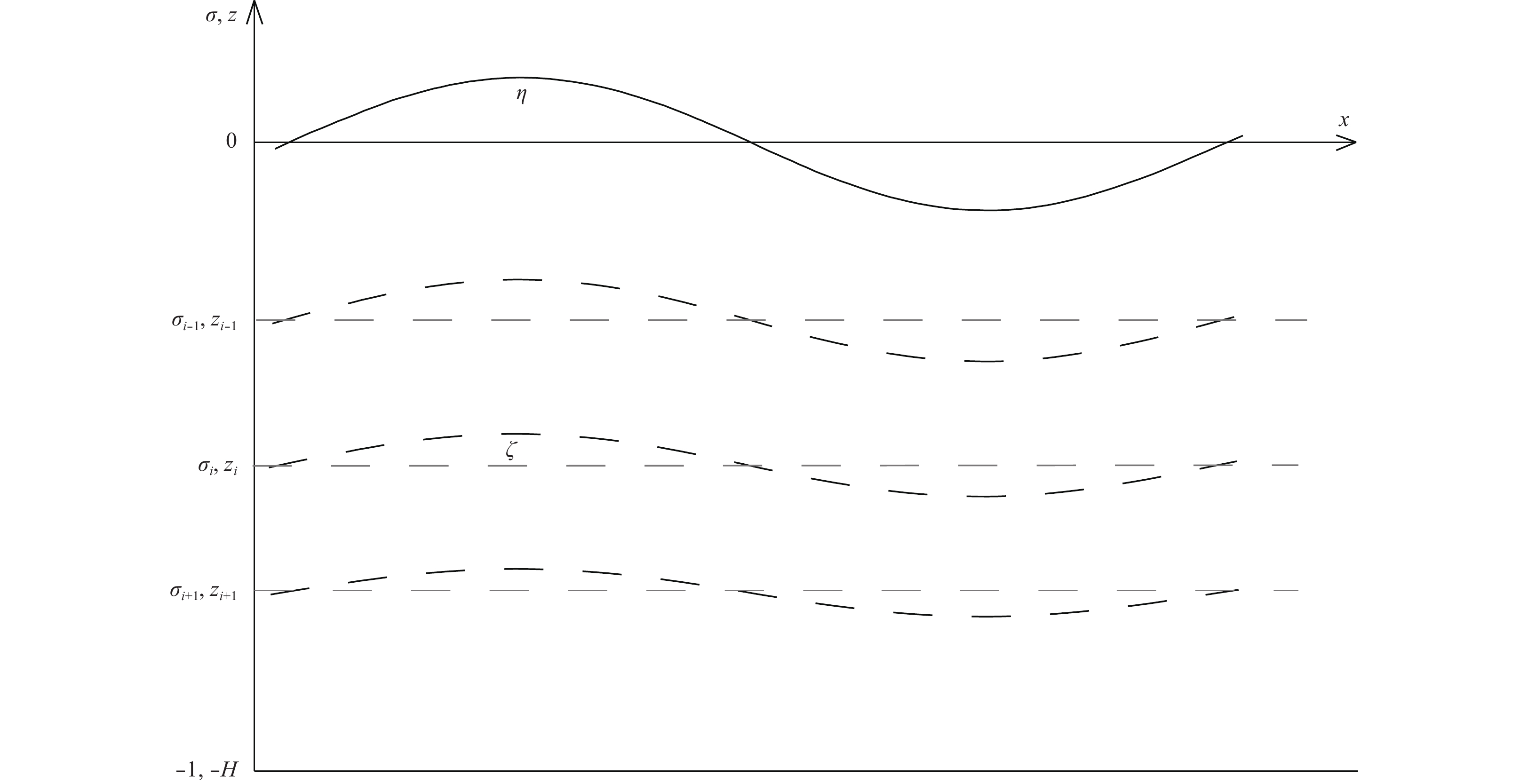
Longuet-Higgins (1969) also provided another description of Stokes velocity that intrigues an understanding of the residual velocity in sigma coordinates. For a one-dimensional progressive gravity wave propagating along the x-direction, the water column is considered to consist of many vertical layers, each fluctuating around a mean depth, zi, like the free surface (Fig. 1). The Stokes drift (or transport) below a free wave surface within the fluid is the mass carried forward by the wave crests plus the mass deficiency carried backward by the troughs, that is, the time mean value of the product of the velocity u (the velocity in the x-direction) and the vertical displacement (ζ) of the wave surface around the mean depth, $ \overline {u\left( {{z_{{i}}} + \zeta } \right)\zeta } $. The Stokes velocity is the vertical differential of the Stokes drift:
Figure
1.
Schematic of sigma coordinates and free wave surfaces of a two-dimensional wave. Solid bold line shows the water surface, and η is the amplitude. Bold dashed lines represent wave surfaces within the fluid, and ζ is the amplitude around a mean depth zi. For shallow water waves, the depths of the sigma layers coincide with the free wave surface.
On the right-hand side of the equation, the two terms are the horizontal and vertical components of the Stokes velocity, corresponding to those in Eq. (3).
2.2
Residual velocity at a sigma layer
The sigma residual velocity is the time average of the velocity at a sigma layer, u(σi) after several cycles of oscillatory motion (here we assume a single frequency motion):
Because the depth of sigma layers varies with time, the residual velocity is located at the mean depth of sigma layers. According to the sigma coordinate transformation, the depth of a sigma layer is
The first term on the right-hand side of the equation is the mean depth of the sigma layer (i.e., zi) if the mean water surface elevation is negligible compared to the mean water depth (i.e., $ \bar \eta \ll H$), and the second term is the temporal variation of the depth of the sigma layer, which indicates that the amplitude of the fluctuation of the sigma layer decreases linearly from η at the surface to zero at the bottom. Assuming that the sea surface fluctuation is small compared to the mean water depth (i.e., $ \eta \ll H$), the first-order approximation of the time-mean velocity of a sigma layer, as given by Cheng et al. (2013), is
This equation shows that the residual velocity of a sigma layer equates to a Eulerian residual velocity ($ \bar u\left( {{z_i}} \right)$) at the mean depth of the sigma layer plus a velocity (i.e., the second term on the right-hand side) that represents the change of velocity in the vertical direction. This velocity has a similar form to the vertical component of the Stokes velocity (see Eq. (4)), and the two velocities may be equivalent if $ \left( {1 + \sigma } \right)\eta = \zeta $.
On the basis of the linear wave theory, in a shallow water region (H/L≤1/20, where L is wave length), the distance of the vertical motion of water particles, ζ, decreases linearly with depth (Dean and Dalrymple, 1991):
where zi/H denotes normalized water depth and is an analogues of σ. This result shows that for shallow water waves, the vertical displacement of water particles within the water column coincides with the sigma layers (i.e., the sigma layers represent the water wave surfaces). Therefore, the sigma residual velocity is the sum of the Eulerian residual velocity and the vertical component of the Stokes velocity, i.e.,
In this sense, the sigma residual velocity can considered as a semi-Lagrangian velocity.
In medium and deep water regions, where H/L>1/20, the distance of the vertical motion of water particles decreases with depth faster than in shallow water regions (Dean and Dalrymple, 1991). The thickness of the sigma layer is less than the distance of the vertical motion of water particles near the surface, but larger near the bottom. As a consequence, the sigma layers do not coincide with the water wave surfaces. However, a non-uniform vertical distribution of sigma layers can be designed to allow the variation of the sigma layer to match the vertical displacement of water particles. By this means, the sigma residual velocity can represent a semi-Lagrangian velocity in medium- and deep-water regions.
2.3
Discrete forms of Stokes velocity
If the sigma layers coincide with the wave surfaces within the fluid, the Stokes velocity can be expressed using the sigma velocity. The Stokes transport beneath a sigma layer (σi) is the product of the velocity and the depth of the sigma layer, i.e., $ \overline {u\left( {x,{\sigma _{{i}}}} \right)\left( {1 + {\sigma _{{i}}}} \right)\eta } $, and the Stokes velocity is written in a discrete form:
where dσ=σ1–1–σi. This equation indicates that the Stokes velocity at a sigma layer is the Stokes transport within the sigma layer (from σi–0.5 to σi+0.5) divided by the thickness of the sigma layer.
According to Eq. (4), if we assume that $ \dfrac{{\partial u\left( {x,z} \right)}}{{\partial z}} \approx \dfrac{{\partial u\left( {x,\sigma } \right)}}{{H\partial \sigma }}$, the vertical component of the Stokes velocity is written as:
Note that $ \dfrac{{\overline {u\left( {x,{\sigma _{{i}}}} \right)\eta } }}{H} = \dfrac{{\overline {u\left( {x,{\sigma _{{i}}}} \right)\left( {1 + {\sigma _{{i}}}} \right)\eta } }}{{\left( {1 + {\sigma _{{i}}}} \right)H}}$, where the numerator is the Stokes transport below a sigma layer, and the denominator is the thickness of the water column below the sigma layer. According to the definition of Stokes velocity (i.e., Eq. (4)), $ \overline {u\left( {x,{\sigma _{{i}}}} \right)\eta } /H$ (or uSh) represents the depth-mean Stokes velocity of the water column beneath the sigma layer σi. The discrete forms of Stokes velocity indicate that the resolution of the sigma layer also influences the calculation of residual velocities in sigma layers. Increasing the number of sigma layers helps reduce computing errors for the vertical gradients of velocity and Stokes transport.
Equation (9) further indicates that the sigma residual velocity is related to the Lagrangian residual velocity, $ {\bar u_{\rm L}}$ as
Although the two components of Stokes velocity typically have the same order of magnitude, the magnitude of uSv could be one order smaller than that of uSh in a narrow tidal channel in which the lateral variability is negligible. The two Stokes velocity components are scaled as follows. The tidal current velocity has a logarithmic profile:
$$u\left( z \right) = \frac{{{u_*}}}{\kappa }{\rm{ln}}\left( {\frac{{D + z}}{{{z_0}}}} \right),$$
(15)
where u* is the friction velocity, κ is the von Karman constant (= 0.41), and z0 is the bottom roughness length. As shown earlier, the water wave surface fluctuation decreases linearly with depth: $ {{\zeta }} = \dfrac{{D + z}}{D}\eta $. Thus, the scale of the vertical component of the Stokes velocity is
The magnitude of z0 is $ O\left( {{{10}^{ - 3}}} \right)$ m, and the magnitude of D is $ O\left( {{{10}}} \right)$ m for a coastal tidal channel. The denominator has a range of 1~10 at depths from 3z0–D to 0, such that the depth-averaged ratio has an order of $ O\left( {0.1} \right)$, indicating that the vertical component is a minor component of the Stokes velocity.
Another argument of the scale of the ratio can be obtained using the depth-averaged Eq. (15):
The friction velocity is related to the depth-averaged velocity through the drag coefficient, CD: $ {u_*} = \dfrac{{\sqrt {{C_D}} }}{H}\displaystyle \int \nolimits_{{z_0} - D}^0 u\rm{d}z$. The ratio becomes
This result implies that the ratio is not related to tidal amplitude and is a characteristic parameter of tidal channels. Given a typical value of CD, 0.002 5, the ratio is about 0.12. Furthermore, Eq. (9) shows that if the magnitude of the sigma residual velocity is similar to that of the Stokes velocity, uSv can be neglected and the sigma residual velocity approximates the Eulerian velocity.
2.5
Residual transport velocity at a sigma layer
Robinson (1981) defined a residual transport velocity, $ {\bar U_T}$ that is the time mean water transport at a specific location divided by the time mean water depth, namely the residual velocity required to transport, within the mean depth, the same volume of water that passes the location:
The residual velocity is considered a Eulerian residual transport velocity (Zimmerman, 1979; Feng et al., 1986b; Jiang and Feng, 2011) because the mass transport is measured at a fixed point. However, Zimmerman (1979) showed that the first term on the farmost right hand side is the Eulerian residual velocity and the second term is Stokes velocity, resulting in that $ {\bar U_T}$ is equal to Lagrangian residual velocity. To resolve this dilemma, he pointed out that the equality rests heavily on the assumption of a spatially uniform velocity field.
To have a better understanding of $ {\bar U_T}$, the residual transport velocity at a sigma layer (hereafter referred to as sigma residual transport velocity) is defined as
The sigma residual transport velocity is the sum of sigma residual velocity and the depth-mean Stokes velocity beneath the sigma layer (or the horizontal component of the Stokes velocity at the sigma layer) and is located at the mean depth of the sigma layer. Substituting Eq. (9) into Eq. 22 results in
Thus, the sigma residual transport velocity is a first-order approximation to the Lagrangian residual velocity under the assumption that $ \eta \ll H$.
Taking the depth-average for Eq. (22) gives the residual transport velocity of the entire water column in sigma coordinates,
This equation is similar to that defined in the z-coordinate, i.e., Eq. (21), except for the first term on the right-hand side of equation. Here, it is the depth-mean sigma residual velocity, whereas it is the depth-mean Eulerian residual velocity in Eq. (21). Although depth-mean velocity is independent of depth, its location is at the mean depth of the water column. If the water column oscillates with waves, the mean water depth is not fixed, and, as a consequence, the depth-mean velocity is a sigma velocity rather than a Eulerian velocity. In the second term on the right-hand side, the water flux in this term is the covariance of the water surface elevation and the depth-mean velocity (not the velocity at the water surface), so that this term is not the depth-mean Stokes velocity, but rather the horizontal component of the depth-mean Stokes velocity. Equation (9) shows that the depth-mean sigma residual velocity (the first term) is the sum of the depth-mean Eulerian residual velocity and the vertical component of the depth-mean Stokes velocity. Combining the horizontal component of the depth-mean Stokes velocity (the second term) with the depth-mean sigma residual velocity leads to a result that the right hand side of Eq. (24) equates the Lagrangian residual velocity although the physical meaning of those terms are different to previous studies. However, we should be aware of the fact that “only in certain circumstances are magnitude and direction of residual transport velocity equal to its Lagrangian counterpart, but never will they be conceptually the same” (Zimmerman, 1979). In this study, the equality of sigma residual transport velocity and Lagragain residual velocity results from the highly simplified assumptions for the one-directional progressive wave.
The theoretical analysis of Stokes velocity and sigma residual velocity is based on a minimization of the lateral variability. When the tidal channel cannot be reduced to breadth-averaged two-dimensional channel, the second term on the right hand side of Eq. (2) is effective, such that the relationship between sigma residual velocity and Stokes velocity built on the assumption that the x-component of Stokes transport is the covariance of wave surface elevation and velocity fluctuation will be invalid. For a wide estuary channel, if the cross-section is divided into multiple subregions of which the vertical levels use the σ–coordinates (a method developed by Lerczak et al. (2006)), the sigma residual transport velocity of those subregions also contains a portion of Stokes velocity and is not equal to the Lagrangian velocity. The physical meaning of residual velocities in the cross-section needs careful interpretation and further exploration.
3.
Numerical experiments
The results of the theoretical analysis were tested using a generic numerical model that configures a simplified tidal channel. A series of numerical experiments were conducted to validate the theoretical analysis and extend it to large ratios of tidal amplitude and mean water depth.
3.1
Model configuration
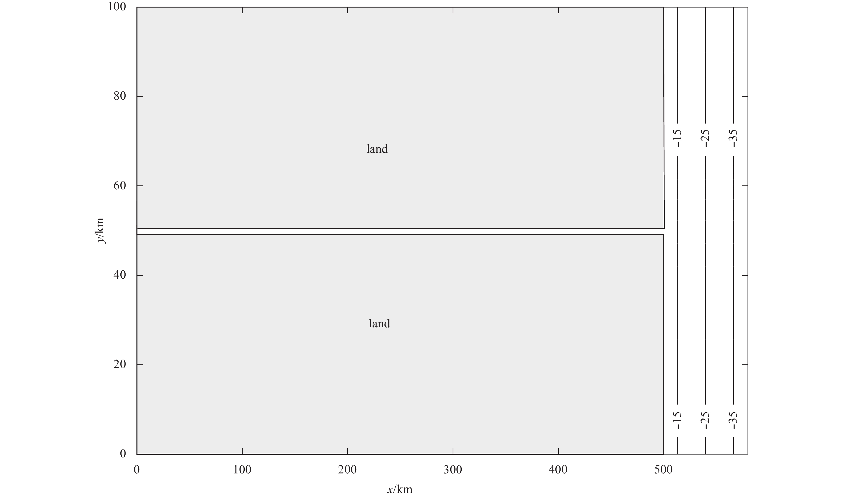
The generic model is based on the Regional Ocean Modeling System, which is a free-surface, hydrostatic, primitive-equations ocean model that uses stretched, terrain following vertical coordinates and orthogonal curvilinear horizontal coordinates on an Arakawa C-grid (Haidvogel et al., 2000; Shchepetkin and McWilliams, 2005). The model domain is designed as a tidal channel-shelf system with a straight tidal channel and a sloped continental shelf (Fig. 2). The channel is 500 km long and has no along-channel bottom slope to minimize bottom bathymetric effects. The long channel is used to allow tides to gradually dissipate. The cross-channel section has a rectangular shape with a depth of 10 m and a width of 600 m. The continental shelf is 80 km wide and has a fixed cross-shelf slope of 0.05%. The salinity and temperature are homogeneous throughout the model domain. A two-equation turbulence closure, k–ω, is used to calculate vertical mixing. The bottom shear stress is calculated using the quadratic dependence with a drag coefficient of 0.002 5.
Figure
2.
Schematic of the numerical model domain and bathymetry.
The model grid is 240 (along-channel, x-direction) by 80 (cross-channel, y-direction) by 20 (vertical, z-direction) cells. The river has 200 grid cells along the channel and 1 grid cell across the channel. The small number of cross-channel cells is designed to minimize the effects of lateral processes. The along-channel grid size increases exponentially from the estuary’s mouth (~100 m) to its head (~12 km), providing a highly resolved region near the mouth. The vertical dimension is discretized with 20 uniform sigma layers. A semidiurnal tide (S2) is imposed at the eastern boundary, and a total of 15 experiments were conducted with tidal amplitudes ranging from 1 to 15 m, with intervals of 1 m. In the experiments, when the offshore tides propagated to the coast, the tidal amplitudes were reduced and had a range of 1 to 5 m at the mouth of the channel.
3.2
Characteristics of residual velocities
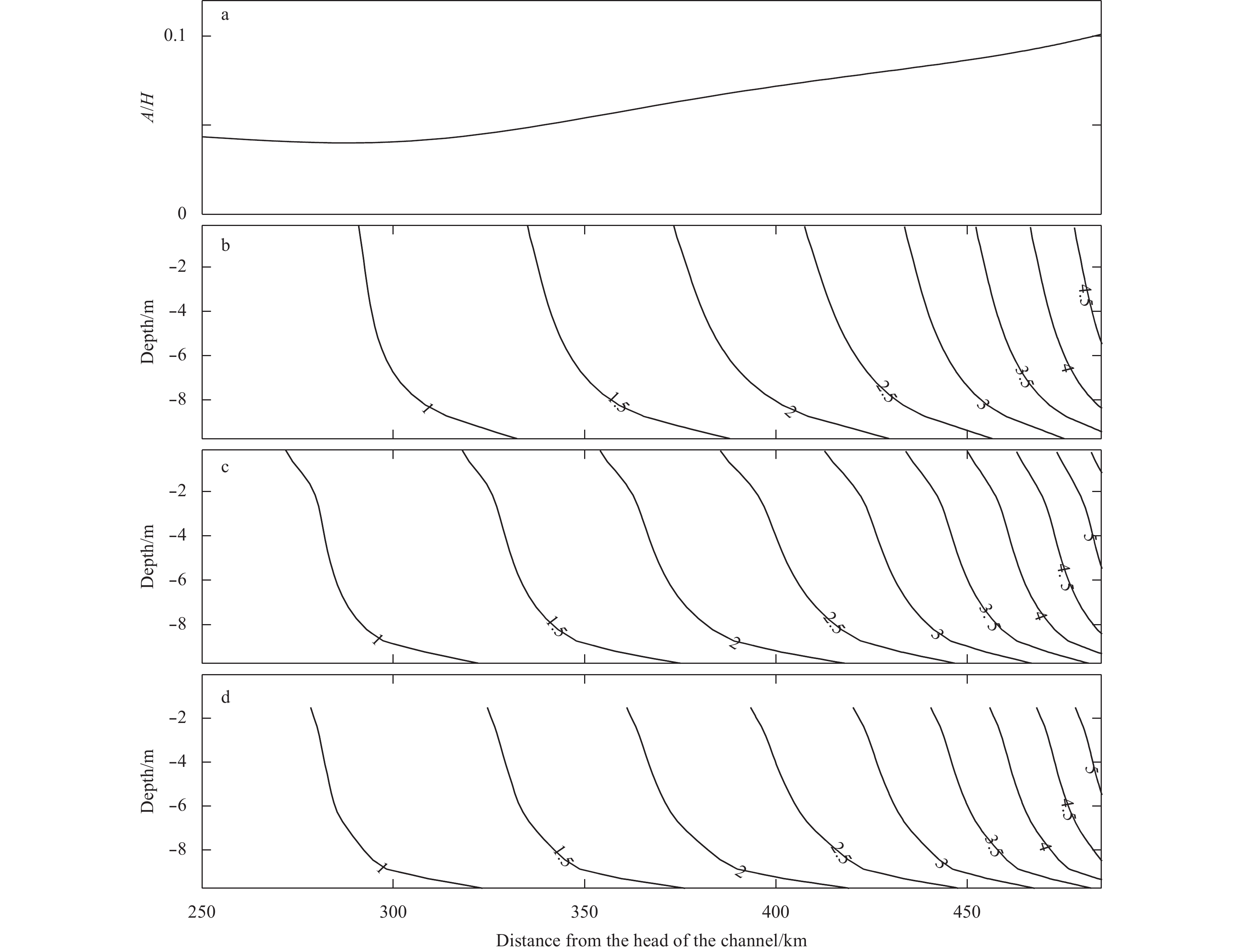
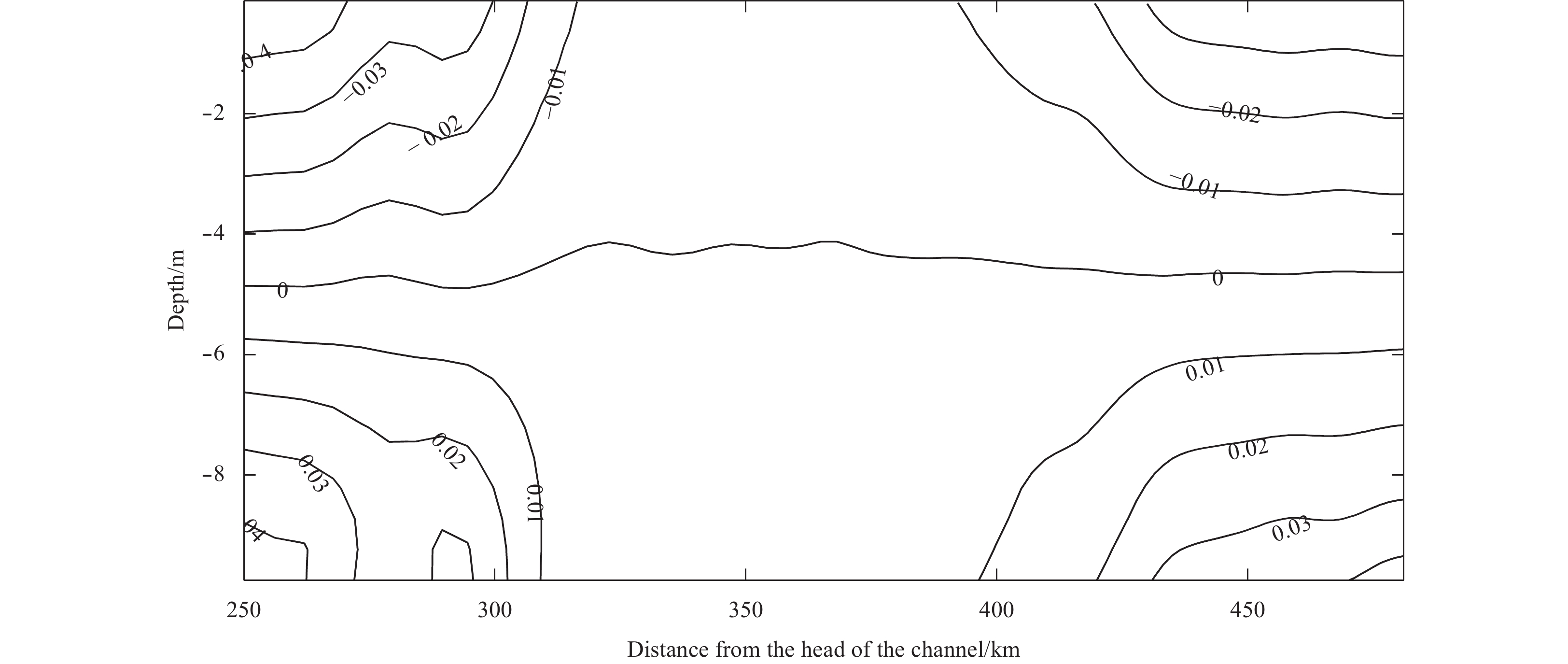
The results of the experiment with a 1-meter tide at the eastern open boundary are used here to illustrate the residual flows in the tidal channel. The tidal amplitudes (A) obtained using harmonic analysis were small compared to the mean water depth (Fig. 3a), satisfying the assumption (i.e., $ \eta \ll H$) for the theoretical analysis of sigma velocity, and gradually decreased from the mouth toward the head of the channel, showing that bottom friction retards the propagation of the tide wave. The channel section from 250 to 490 km, where the tide was relatively strong, was selected for analysis to reduce the influence of computation errors on residual velocities. Corresponding to the change of tidal amplitude, the magnitude of sigma residual velocity also decreased landward, and the flow direction was seaward (positive values) (Fig. 3b). Using Eq. (9), the Eulerian residual velocity was obtained by subtracting the vertical component of Stokes velocity from the sigma residual velocity and showed a similar pattern to the sigma residual velocity (Fig. 3c). The magnitude of the Eulerian residual velocity was slightly larger than the sigma residual velocity because of the landward vertical component of the Stokes velocity (Fig. 4b). The Eulerian residual velocity could also be directly calculated beneath the low tidal water level (here, the surface layer of 1.5 m was excluded in the computation, Fig. 3d). The two Eulerian residual velocities obtained from the two methods agreed well with each other, thus confirming Eq. (9) .
Figure
3.
Along-channel distributions of the ratio of tidal amplitude (a), A, to mean water depth; H, sigma residual velocity (b); the Eulerian residual velocity obtained by subtracting the vertical component of Stokes velocity from the sigma residual velocity (c); and the Eulerian residual velocity calculated beneath the low tide (d). Positive values indicate seaward flow, and the channel mouth is located at a distance of 500 km. The velocities are given in cm/s.
Figure
4.
Along-channel distributions of Stokes velocity (a), the vertical component of Stokes velocity (b), the horizontal component of Stokes velocity (c), and the difference between a and c. (d). Negative values indicate landward flow, and the channel mouth is located at a distance of 500 km. The velocities are given in cm/s.
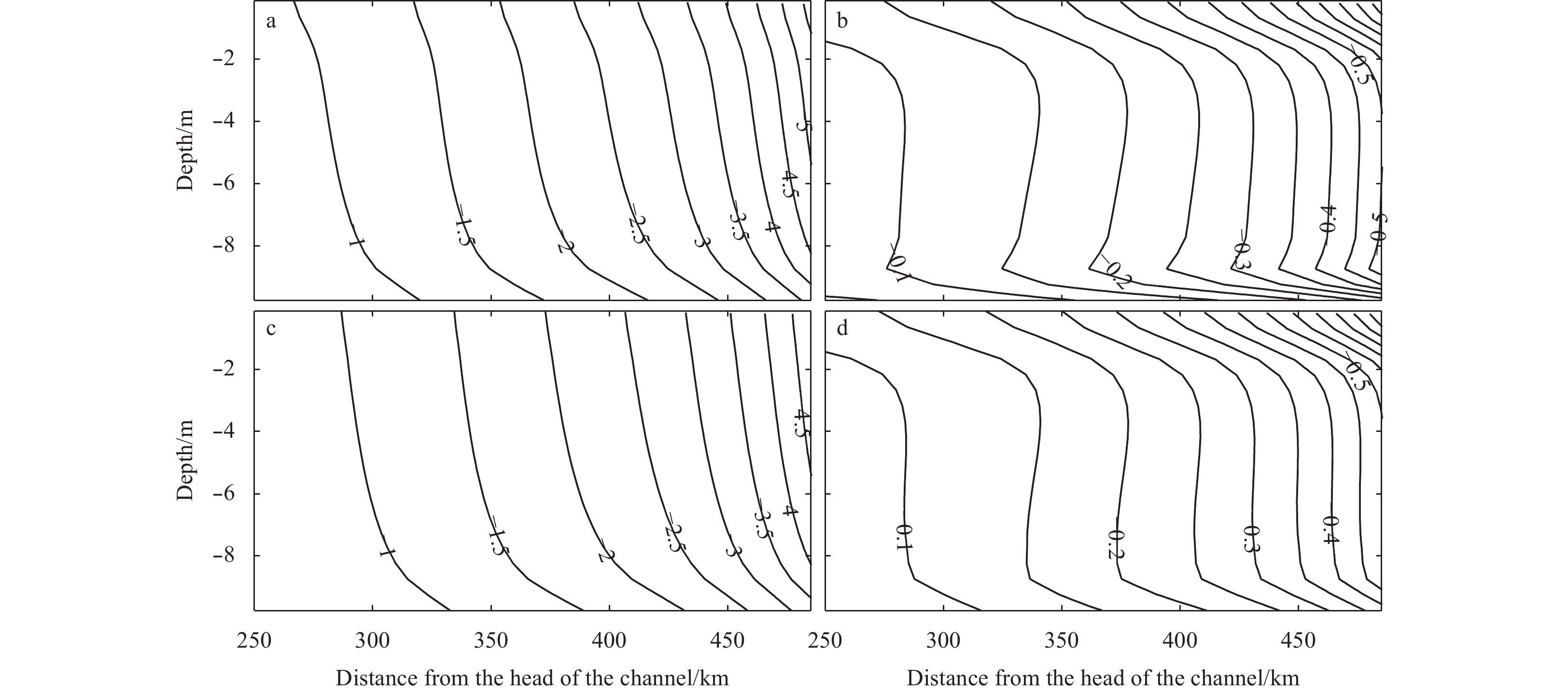
The Stokes velocity and its two components were computed using the discrete forms (i.e., Eqs (11)–(13)). The three velocities were landward (Figs 4a, b, c), and the vertical component was one order of magnitude smaller than the horizontal component, supporting the scale analysis. The vertical component of the Stokes velocity can also be obtained by subtracting the horizontal component from the Stokes velocity (Fig. 4d). The two vertical components showed similar magnitudes and distributions. Relative large differences appeared near the bottom, possibly because the computation error of the vertical velocity gradient are large near the bottom. Increasing the number of sigma layers might reduce the computation errors. The comparison of the Stokes velocities confirmed the consistency of the discrete formulae.
The sigma residual transport velocity was calculated using Eq. (22), and showed a small magnitude with an order of O (10–2) cm/s (Fig. 5). The flow has a two-layer structure, with landward flow near the surface and seaward flow near the bottom. The analytical model for two-dimensional tidal channels shows that the Lagrangian residual flow has a two-layer structure if the non-dimensional parameter d0 ($ = H/\sqrt {2{K_m}/\omega } $, where Km is the vertical eddy viscosity, ω is the tidal frequency) is less than 5 (Ianniello, 1977). Using the depth-mean vertical eddy viscosity from the numerical model output, d0 can be estimated, and has a range from 0.8 to 1.2 in the channel from 250 to 490 km. The pattern of residual transport velocity is consistent with that of Lagrangian residual flow predicted from the analytical solution. Under the assumption of a small tidal amplitude, the sigma residual transport velocity approximates the Lagrangian residual velocity.
Figure
5.
Along-channel distribution of sigma residual transport velocity. Positive values indicate seaward flow, and the channel mouth is located at a distance of 500 km. The velocities are given in cm/s.
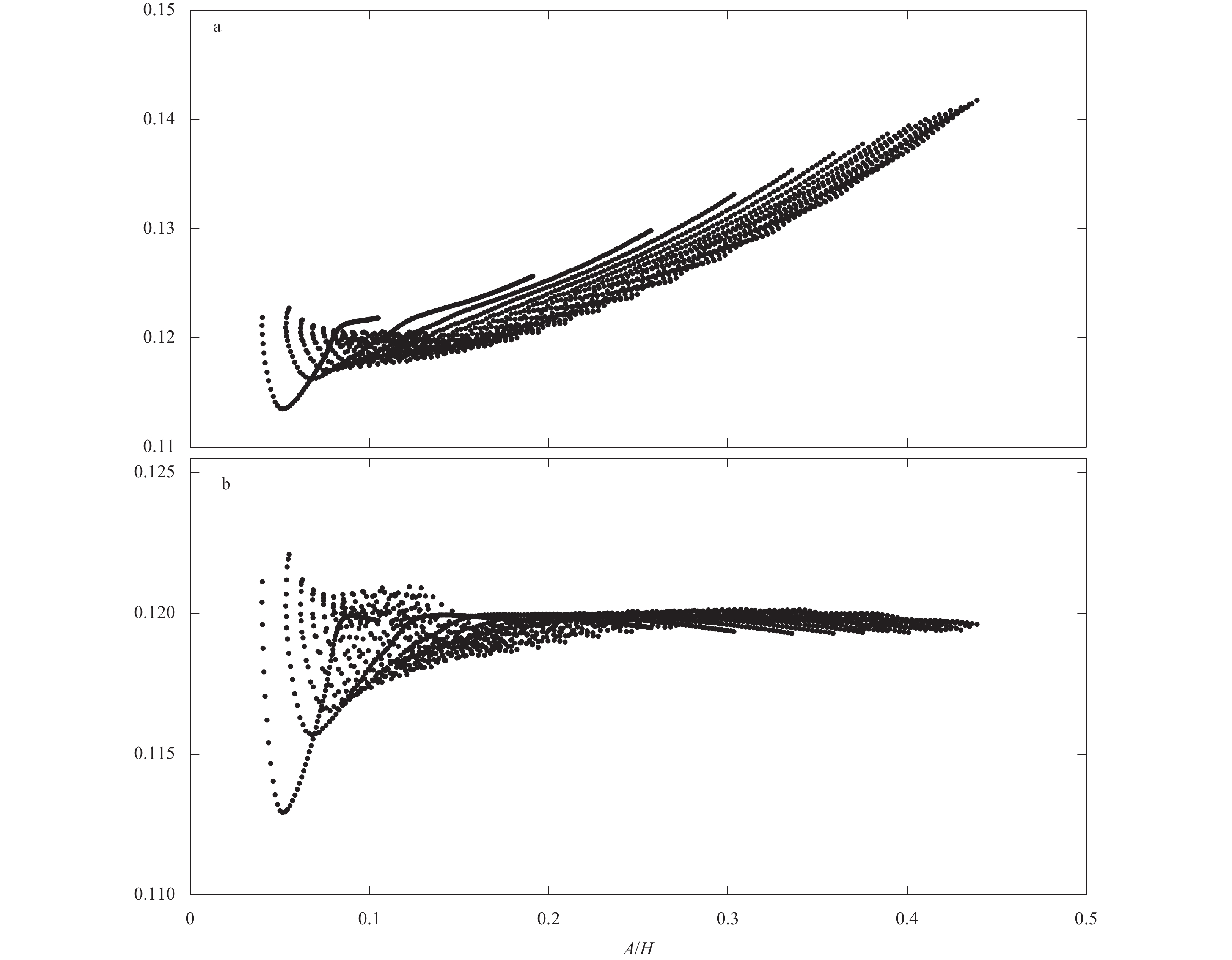
The vertical component of Stokes velocity can be calculated using the derivative form (i.e., Eq. (10)) and the discrete form (i.e., Eq.(12)). To examine the validity of the two formulae, the vertical component of the Stokes velocity was compared with the horizontal component, because the preceding scale analysis has shown that the ratio of the vertical and horizontal components is about 0.12 with a CD of 0.002 5, and is independent of tidal amplitudes. Combining the results of all 15 experiments, the ratio of the two components was about 0.12 for small tidal amplitude to mean water depth ratios (A/H), and tended to exponentially increase with larger A/H when the vertical component of Stokes velocity was calculated using the derivative form (Fig. 6a). By comparison, the ratio remained constant with A/H when the vertical component of Stokes velocity was calculated using the discrete form (Fig. 6b). In the calculation of the vertical component of Stokes velocity using Eq. (10), the vertical gradient of velocity was calculated using the sigma velocity and interpolated/extrapolated to the mean depths of sigma layers. Computation errors may be significant when tidal amplitude is large compared to the mean water depth. However, the discrete form of the vertical component of Stokes velocity avoided the need to interpolate/extrapolate the vertical gradient of velocity and provided a reliable ratio of the two components. Therefore, the discrete form of the vertical component of Stokes velocity is less sensitive to tidal amplitudes.
Figure
6.
Ratio of the vertical and horizontal components of Stokes velocity as a function of the ratio of tidal amplitude (A) to mean water depth (H). The vertical component of the Stokes velocity was calculated using the derivative form (a) and the discrete form (b).
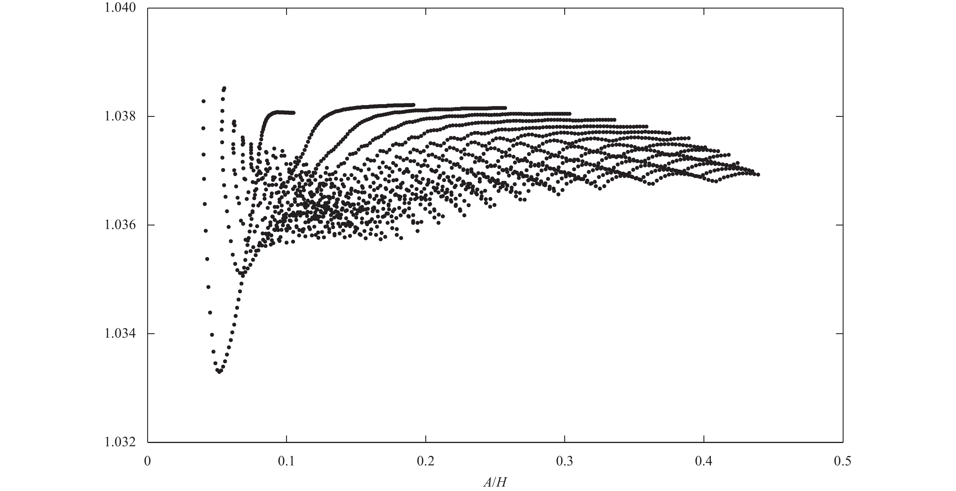
To further examine whether the discrete formula provides a reasonable estimation of the vertical component of Stokes velocity, the difference between the Stokes velocity and its horizontal component was computed and treated as the “true” vertical component. Next, the vertical component calculated using the discrete form was compared with the “true” vertical component (Fig. 7). The ratio of the two vertical components was about 1.037 and was insensitive to tidal amplitude, confirming the validity of the discrete formula. Nonetheless, the 3.7% difference suggests that the discrete formula slightly overestimates the vertical component. The computation errors mostly resulted from the assumption $ \dfrac{{\partial u\left( {x,z} \right)}}{{\partial z}} \approx \dfrac{{\partial u\left( {x,\sigma } \right)}}{{H\partial \sigma }}$.
Figure
7.
Ratio of the vertical components of Stokes velocity calculated with the discrete form, and the difference between the Stokes velocity and its horizontal component as a function of the ratio of tidal amplitude (A) to mean water depth (H).
A comparison of Eulerian residual velocities was conducted to examine whether Eq. (9) can be extended to large A/H. The Eulerian residual velocity directly calculated in the low water column beneath the low tide level was considered the “true” Eulerian residual velocity. The Eulerian residual velocity was also computed for the low water column according to Eq. (9), as the difference between the sigma residual velocity and the vertical component of the Stokes velocity. The ratio of the depth-mean values of the two Eulerian residual velocities was calculated and showed no clear relationship with A/H (Fig. 8). The ratio was about 1.0, with a variation of less than 0.5%. This result indicates that it is possible to generalize the relationship stated by Eq. (9) that the sigma residual velocity is the sum of the Eulerian residual velocity and the vertical component of the Stokes velocity. Because the sigma residual transport velocity typically has a much smaller magnitude than the Eulerian and Stokes velocities (two order smaller in the experiment with a 1 m tide, see Section 3.2), it could be affected by the 0.5% difference and contain a portion of the Stokes velocity.
Figure
8.
Ratio of the Eulerian residual velocity obtained by subtracting the vertical component of Stokes velocity from the sigma residual velocity and the Eulerian residual velocity directly calculated beneath the low tide level as a function of the ratio of tidal amplitude (A) to mean water depth (H). The ratio is the depth-mean over the water column beneath the low tidal level.
Based on the framework of Stokes velocity developed by Longuet-Higgins (1969), this study has attempted to understand the physical meaning of the residual velocities in sigma coordinates in narrow tidal channels that can be reduced to breadth-averaged two-dimensional channels. For shallow water waves, the vertical temporal variation of sigma layers coincides with the vertical displacement of water particles within the water column that decreases linearly with depth, such that the sigma layers represent the water wave surfaces. Using the idea that the Stokes transport below a free wave surface within the fluid is the mass difference between the mass carried forward and backward by the wave, the Stokes velocity and its vertical and horizontal components can be expressed in discrete forms with the sigma velocity, which provides a convenient method for calculating the Stokes velocity and its components.
Under the assumption of a low ratio of tidal amplitude to mean water depth, the Taylor expansion showed that the time-mean velocity of a sigma layer (i.e., the sigma residual velocity) is the sum of the Eulerian residual velocity and the vertical component of the Stokes velocity at the mean depth of the sigma layer. A series of generic numerical experiments confirmed that this relationship can be extended to a large ratio of the tidal amplitude to the mean water depth. Therefore, the sigma residual velocity can be referred to as a semi-Lagrangian residual velocity because it contains part of the Stokes velocity.
Scaling analysis showed that the vertical component of Stokes velocity is about O(0.1) of the horizontal component and is independent of tidal amplitude. This relation was confirmed by numerical results, and further indicates that if the sigma residual velocity has the same magnitude as the Stokes velocity, the vertical component of the Stokes velocity can be neglected, such that the sigma residual velocity is an approximation of the Eulerian residual velocity.
The residual transport velocity was considered the sum of Eulerian residual velocity and Stokes velocity, i.e., an approximation of Lagrangian residual velocity. While the analysis of sigma velocity showed that the residual transport velocity of a sigma layer is the sum of sigma residual velocity and the depth-mean Stokes velocity beneath the sigma layer (i.e., the horizontal component of the Stokes velocity) and also approximates the Lagrangian residual velocity. The result updated the understanding of the residual transport velocity.
Acknowledgements
We are grateful to the anonymous reviewers for their insightful comments that helped to improve this work.
Bowden K F. 1963. The mixing processes in a tidal estuary. International Journal of Air and Water Pollution, 7: 343–356
[2]
Cheng Peng, de Swart H E, Valle-Levinson A. 2013. Role of asymmetric tidal mixing in the subtidal dynamics of narrow estuaries. Journal of Geophysical Research: Oceans, 118(5): 2623–2639. doi: 10.1002/jgrc.20189
[3]
Dean R G, Dalrymple R A. 1991. Water Wave Mechanics for Engineers and Scientists. Singapore: World Scientific Press, 80-83
[4]
Dyer K R, Ramamoorthy K. 1969. Salinity and water circulation in the Vellar estuary. Limnology and Oceanography, 14(1): 4–15. doi: 10.4319/lo.1969.14.1.0004
[5]
Feng Shizuo, Cheng R T, Xi Pangen. 1986a. On tide-induced Lagrangian residual current and residual transport: 1. Lagrangian residual current. Water Resources Research, 22(12): 1623–1634. doi: 10.1029/WR022i012p01623
[6]
Feng Shizuo, Cheng R T, Xi Pangen. 1986b. On tide-induced Lagrangian residual current and residual transport: 2. Residual transport with application in South San Francisco Bay, California. Water Resources Research, 22(12): 1635–1646. doi: 10.1029/WR022i012p01635
[7]
Giddings S N, Monismith S G, Fong D A, et al. 2014. Using depth-normalized coordinates to examine mass transport residual circulation in estuaries with large tidal amplitude relative to the mean depth. Journal of Physical Oceanography, 44(1): 128–148. doi: 10.1175/JPO-D-12-0201.1
[8]
Haidvogel D B, Arango H G, Hedstrom K, et al. 2000. Model evaluation experiments in the North Atlantic Basin: simulations in nonlinear terrain-following coordinates. Dynamics of Atmospheres and Oceans, 32(3/4): 239–281. doi: 10.1016/S0377-0265(00)00049-X
[9]
Ianniello J P. 1977. Tidally induced residual currents in estuaries of constant breadth and depth. Journal of Marine Research, 35(4): 755–786
[10]
Jiang Wensheng, Feng Shizuo. 2011. Analytical solution for the tidally induced Lagrangian residual current in a narrow bay. Ocean Dynamics, 61(4): 543–558. doi: 10.1007/s10236-011-0381-z
[11]
Jiang Wensheng, Feng Shizuo. 2014. 3D analytical solution to the tidally induced lagrangian residual current equations in a narrow bay. Ocean Dynamics, 64(8): 1073–1091. doi: 10.1007/s10236-014-0738-1
[12]
Kjerfve B. 1975. Velocity averaging in estuaries characterized by a large tidal range to depth ratio. Estuarine and Coastal Marine Science, 3(3): 311–323. doi: 10.1016/0302-3524(75)90031-6
[13]
Kuo A Y, Hamrick J M, Sisson G M. 1990. Persistence of residual currents in the James River estuary and its implication to mass transport. In: Cheng R T, ed. Residual Currents and Long-term Transport. New York, NY: Springer, 389–401.
[14]
Lerczak J A, Geyer W R, Chant R J. 2006. Mechanisms driving the time-dependent salt flux in a partially stratified estuary. Journal of Physical Oceanography, 36(12): 2296–2311. doi: 10.1175/JPO2959.1
[15]
Longuet-Higgins M S. 1969. On the transport of mass by time-varying ocean currents. Deep Sea Research and Oceanographic Abstracts, 16(5): 431–447. doi: 10.1016/0011-7471(69)90031-X
[16]
Rattray M Jr, Dworski J G. 1980. Comparison of methods for analysis of the transverse and vertical circulation contributions to the longitudinal advective salt flux in estuaries. Estuarine and Coastal Marine Science, 11(5): 515–536. doi: 10.1016/S0302-3524(80)80004-1
[17]
Robinson I S. 1981. Tidal vorticity and residual circulation. Deep Sea Research Part A. Oceanographic Research Papers, 28(3): 195–212. doi: 10.1016/0198-0149(81)90062-5
[18]
Shchepetkin A F, McWilliams J C. 2005. The regional oceanic modeling system (ROMS): a split-explicit, free-surface, topography-following-coordinate oceanic model. Ocean Modelling, 9(4): 347–404. doi: 10.1016/j.ocemod.2004.08.002
[19]
Zimmerman J T F. 1979. On the Euler-Lagrange transformation and the Stokes’ drift in the presence of oscillatory and residual currents. Deep Sea Research Part A. Oceanographic Research Papers, 26(5): 505–520
Xiaoxuan Sheng, Qi Quan, Jinzhen Yu, et al. Tide-induced Lagrangian residual velocity and dynamic analysis based on field observations in the inner Xiangshan Bay, China. Acta Oceanologica Sinica, 2022, 41(10): 32. doi:10.1007/s13131-022-2007-3
2.
Xiaoxuan Sheng, Xinyan Mao, Jinzhen Yu, et al. Modeling Lagrangian residual velocity in a tide-dominated long-narrow bay: case study of the inner Xiangshan Bay. Estuarine, Coastal and Shelf Science, 2022, 278: 108088. doi:10.1016/j.ecss.2022.108088
3.
Isaac Rodríguez-Padilla, Bruno Castelle, Vincent Marieu, et al. Wave-Filtered Surf Zone Circulation under High-Energy Waves Derived from Video-Based Optical Systems. Remote Sensing, 2021, 13(10): 1874. doi:10.3390/rs13101874
4.
Yi-chang Yu, Bo-heng Shen, Zhi-wei Li, et al. Proceedings of the International Field Exploration and Development Conference 2023. Springer Series in Geomechanics and Geoengineering, doi:10.1007/978-981-97-0464-4_26
Figure 1. Schematic of sigma coordinates and free wave surfaces of a two-dimensional wave. Solid bold line shows the water surface, and η is the amplitude. Bold dashed lines represent wave surfaces within the fluid, and ζ is the amplitude around a mean depth zi. For shallow water waves, the depths of the sigma layers coincide with the free wave surface.
Figure 2. Schematic of the numerical model domain and bathymetry.
Figure 3. Along-channel distributions of the ratio of tidal amplitude (a), A, to mean water depth; H, sigma residual velocity (b); the Eulerian residual velocity obtained by subtracting the vertical component of Stokes velocity from the sigma residual velocity (c); and the Eulerian residual velocity calculated beneath the low tide (d). Positive values indicate seaward flow, and the channel mouth is located at a distance of 500 km. The velocities are given in cm/s.
Figure 4. Along-channel distributions of Stokes velocity (a), the vertical component of Stokes velocity (b), the horizontal component of Stokes velocity (c), and the difference between a and c. (d). Negative values indicate landward flow, and the channel mouth is located at a distance of 500 km. The velocities are given in cm/s.
Figure 5. Along-channel distribution of sigma residual transport velocity. Positive values indicate seaward flow, and the channel mouth is located at a distance of 500 km. The velocities are given in cm/s.
Figure 6. Ratio of the vertical and horizontal components of Stokes velocity as a function of the ratio of tidal amplitude (A) to mean water depth (H). The vertical component of the Stokes velocity was calculated using the derivative form (a) and the discrete form (b).
Figure 7. Ratio of the vertical components of Stokes velocity calculated with the discrete form, and the difference between the Stokes velocity and its horizontal component as a function of the ratio of tidal amplitude (A) to mean water depth (H).
Figure 8. Ratio of the Eulerian residual velocity obtained by subtracting the vertical component of Stokes velocity from the sigma residual velocity and the Eulerian residual velocity directly calculated beneath the low tide level as a function of the ratio of tidal amplitude (A) to mean water depth (H). The ratio is the depth-mean over the water column beneath the low tidal level.


 DownLoad:


 DownLoad: