Key Laboratory of Marine Hazards Forecasting, National Marine Environmental Forecasting Center, Ministry of Natural Resources, Beijing 100081, China
2.
Laboratory for Regional Oceanography and Numerical Modeling, Pilot National Laboratory for Marine Science and Technology (Qingdao), Qingdao 266237, China
3.
First Institute of Oceanography, Ministry of Natural Resources, Qingdao 266061, China
4.
College of Oceanic and Atmospheric Sciences, Ocean University of China, Qingdao 266100, China
5.
Key Laboratory for Marine Science and Numerical Modeling, Ministry of Natural Resources, Qingdao 266061, China
6.
IMSG at Environmental Modeling Center, National Centers for Environmental Prediction, National Oceanic and Atmospheric Administration, College Park, MD 20740, USA
Funds:
The National Key Research and Development Program of China under contract No. 2018YFC1407206; the National Natural Science Foundation of China under contract Nos 41821004 and U1606405; the Basic Scientific Fund for National Public Research Institute of China (Shu Xingbei Young Talent Program) under contract No. 2019S06.
Subseasonal Arctic sea ice prediction is highly needed for practical services including icebreakers and commercial ships, while limited by the capability of climate models. A bias correction methodology in this study was proposed and performed on raw products from two climate models, the First Institute Oceanography Earth System Model (FIOESM) and the National Centers for Environmental Prediction (NCEP) Climate Forecast System (CFS), to improve 60 days predictions for Arctic sea ice. Both models were initialized on July 1, August 1, and September 1 in 2018. A 60-day forecast was conducted as a part of the official sea ice service, especially for the ninth Chinese National Arctic Research Expedition (CHINARE) and the China Ocean Shipping (Group) Company (COSCO) Northeast Passage voyages during the summer of 2018. The results indicated that raw products from FIOESM underestimated sea ice concentration (SIC) overall, with a mean bias of SIC up to 30%. Bias correction resulted in a 27% improvement in the Root Mean Square Error (RMSE) of SIC and a 10% improvement in the Integrated Ice Edge Error (IIEE) of sea ice edge (SIE). For the CFS, the SIE overestimation in the marginal ice zone was the dominant features of raw products. Bias correction provided a 7% reduction in the RMSE of SIC and a 17% reduction in the IIEE of SIE. In terms of sea ice extent, FIOESM projected a reasonable minimum time and amount in mid-September; however, CFS failed to project both. Additional comparison with subseasonal to seasonal (S2S) models suggested that the bias correction methodology used in this study was more effective when predictions had larger biases.
Arctic sea ice extent and thickness have substantially decreased when compared to satellite observations available from the late 1970s (Comiso et al., 2008). This is especially apparent in September, when the rate of sea ice extent reduction has increased from (0.032±0.017)×106 km2/a during 1979–1998 to (0.154±0.038)×106 km2/a during 1999–2010 (Stroeve et al., 2012). The extent of multi-year ice showed a sudden decrease from 4.69×10⁶ km2 to 3.61×10⁶ km2 during 2005–2007 (Nghiem et al., 2007). Previous study also noticed that there was a significant reduction in ice thickness, with a rate that reached 0.17 m/a during 2003–2008 (Kwok et al., 2009). At the same time, the ice melting season increased by 20 days in the past 30 years from 1979 to 2009 (Markus et al., 2009).
Under the background of frequent Arctic activities, subseasonal Arctic sea ice predictions have become increasingly important for commercial companies, icebreaker captains, and policy makers, as the spatial distribution of ice extent is key information required for planning cruises several months ahead, and/or identifying safe routes several weeks ahead. However, current dynamical models are still not solid enough for making subseasonal predictions; this is primarily due to errors in the model physics and initial conditions (Blanchard-Wrigglesworth et al., 2015). For sea ice outlook comparisons, model prediction is only marginally better than the linear trend results (Stroeve et al., 2014), and the skill of numerical models in predicting seasonal minimum ice extent is generally comparable to that of statistical methods (Zampieri et al., 2018; Wayand et al., 2019). Due to these facts, sea ice prediction remains quite challenging in Arctic (Liu et al., 2019) and also in Antarctic (Zampieri et al., 2019). To reduce the gap between model predictability and service requirements, previous studies applied bias corrections based on the differences between predictions and observations, which proved to be effective (Meehl et al., 2014; Blanchard-Wrigglesworth et al., 2017; Director et al., 2017).
The first Chinese National Arctic Research Expedition (CHINARE) was conducted in 1999, and the Pacific section was chosen for its investigation domain. Icebreaker Xuelong became the first Chinese research vessel to sail across the Northeast Passage from the Bering Strait to the North Atlantic in the summer of 2012, and it crossed the Central Passage and Northwest Passage in the summer of 2017. In 2013, the China Ocean Shipping (Group) Company (COSCO) initiated the first Chinese commercial cruise from China to Europe and successfully developed it as an operational route. By the summer of 2018, nine research cruises and 22 commercial voyages have been conducted by China in the Arctic region.
In the summer of 2018, subseasonal Arctic sea ice predictions based on two climate models, the First Institute Oceanography Earth System Model (FIOESM v1.0) and the National Centers for Environmental Prediction (NCEP)-Climate Forecast System (CFS v2.0), were carried out to support the ninth CHINARE activities in the Pacific Section and eight COSCO commercial voyages across the Northeast Passage (Fig. 1). The active period was from July to October, when sea ice extent was relative low in the Arctic. Xuelong usually sailed north to 85°N, in order to find large, solid, and continuous ice floes for field scientific experiments. The captain would pay more attention on sea ice concentration (SIC) when Xuelong sailed into multi-year ice zone at a high latitude, because multi-year ice thickness was beyond the ice-breaking ability of Xuelong, under which condition high concentration would increase the risk to be trapped. COSCO commercial ships usually sailed along the coast of Russian Arctic, where sea ice was free from early July. The normal time for ships sailed from the Bering Strait to the Norwegian Sea was about 10–20 d, depending on sea ice condition in the narrow straits or pilotage arrangement of Russian icebreakers. Because most of their commercial ships had no ice-resistance ability, the captains would always prefer to sail in the open water. So the location of sea ice edge (SIE) was amongst the top priorities for the captains.
Figure
1.
The Route of icebreaker Xuelong (solid black line) and COSCO commercial voyages (dashed line in different colors) during summer 2018. The sea ice concentration of August 1, 2018 was illustrated. The date inside brackets after the ship names represented the period they sailed in Arctic.
We proposed a bias correction technology to improve the raw products from two operational prediction models, FIOESM and CFS, and bias corrected products were used to service Arctic voyages navigation, which was the first attempt in China to include this methodology in the official practical services of subseasonal Arctic sea ice prediction. According to the reasons mentioned in the last paragraph, SIC in high latitude and SIE in the marginal area were amongst the top priorities for icebreaker Xuelong and commercial ships. Therefore our assessment focused on the bias of SIC and SIE. In Section 2, operational models and experiments, benchmark forecasts, Subseasonal to Seasonal (S2S) Prediction Project and satellite data are introduced. The methodology of bias correction used in this study is described in Section 3. Model bias and the bias-corrected products are shown in Section 4. The discussion on different initialization dates and comparison with S2S results is presented in Section 5. The summary and conclusions are presented in Section 6.
2.
Models and data
2.1
Models description
FIOESM is the first fully coupled Earth system model that considers the ocean surface wave model by including non-breaking wave-induced vertical mixing (Qiao et al., 2004) into the ocean model. The model components are Community Atmosphere Model Version 3 (CAM3), Community Land Model Version 3.5 (CLM3.5), Los Alamos National Laboratory sea ice model Version 4 (CICE4), Parallel Ocean Program Version 2.0 (POP2.0), and the Marine Science and Numerical Modeling (MASNUM) surface wave model. Further detailed information regarding FIOESM can be found in a previous study (Qiao et al., 2013). A data assimilation scheme based on the Ensemble Adjustment Kalman Filter (EAKF) and Localized Error Subspace Transform ensemble Kalman Filter (LESTKF) was performed to generate the initialization by assimilation of sea surface temperature, sea level anomaly, sea ice concentration, and sea ice thickness (Shu et al., 2015a; Chen et al., 2016). The atmospheric model was initialized from historical control run. The horizontal resolution is a nominal 1° for sea ice products from FIOESM.
The NCEP CFS model is a coupled atmosphere-ocean-land surface-sea ice model. The atmospheric model was based on the NCEP operational global forecast system (GFS) model with improvements, including new radiation and physics (Saha et al, 2010). The horizontal resolution is T126 with 64 hybrid vertical layers. The ocean model is from the Geophysical Fluid Dynamics Laboratory (GFDL) Modular Ocean Model version 4p0d (MOM4, Griffies et al., 2004), with 40 vertical layers. The zonal resolution of MOM4 is 0.5°. The meridional resolution is 0.25° between 10°S and 10°N and gradually increases through the tropics, becoming 0.5° poleward of 30°S and 30°N. The ocean model uses a tripolar grid north of 65°N. The land surface model is the Noah land surface model (Ek et al., 2003), which is imbedded in the GFS. The sea ice model is from the GFDL Sea Ice Simulator with slight modifications, allowing excessive heat from the ocean to store in the sea water instead of overmuch melting the sea ice in winter. There are three layers including two equal layers of sea ice and one (optional) layer of snow with five categories of sea ice thickness (0–0.1 m, 0.1–0.3 m, 0.3–0.7 m, 0.7–1.1 m, and a category greater than 1.1 m). The snow has no heat capacity, the upper ice layer has sensible and latent heat capacity (i.e., a variable temperature/salinity dependent), and the lower ice layer has only sensible (fixed) heat capacity. The base of the ice is fixed at (salinity dependent) the freezing temperature for seawater.
The sea ice dynamics are based on Hunke and Dukowicz (1997) using the elastic-viscous-plastic technique to calculate ice internal stress. The ice strength calculations follow those of Hibler III (1979). The ice thermodynamics are based on a study by Winton (2000). Global Atmospheric, Ocean, and Land Data Assimilation System (GDAS, GODAS, and GLDAS) are used for providing the initial conditions for CFS, including a SIC Nudging scheme for the sea ice initialization in the CFS operational runs (Saha et al., 2014).
2.2
Model experiments
Four reference runs were carried out, initialized on July 1, August 1, and September 1 of each year for 2014, 2015, 2016, and 2017, and then run for 60 days, for the purpose of obtaining the bias of the FIOESM and CFS models. The real forecast experiment for summer 2018 was initialized on July 1, August 1, and September 1, and run for 60 days, in order to predict the sea ice conditions. All experiments were run with 10 ensembles (Table 1). This work was a part of the official sea ice service for the ninth CHINARE and COSCO Northeast Passage voyages, provided by the National Marine Environmental Forecasting Center.
We employed a benchmark forecast as reference to assess the predictive skills of the forecast systems, which was called “climatological trend” forecast (CLIM). This was based on the observed sea ice conditions 30 years previous to the forecast target time. The linear least squares trend was fit to SIC observations from 1988 to 2017 at each grid cell and used to predict SIC values for each day of 2018.
2.4
S2S forecasts
Subseasonal to seasonal forecasts are available on the website https://confluence.ecmwf.int/display/S2S/Models (Vitart et al., 2017). The stored datasets are from year 2015 and initialized once every month. We downloaded predictions of JMA, Meteo France, HMCR, CMA, and ECMWF initialized on July, August and September from 2015 to 2018. Unfortunately, after checking the downloaded data, we found that the predictions in some single month were obviously incorrect for HMCR and CMA, which caused the failure in the mean bias calculation. For Meteo France, the predictions for some year were incomplete and stored time series were less than 60 d. Therefore only JMA and ECMWF predictions were used to compare with the 60 d predictions in this study.
2.5
Satellite dataset
The satellite sea ice concentration (SIC) dataset used in this study is from Advanced Microwave Scanning Radiometer 2 (AMSR2), which has been operating onboard the Global Change Observation Mission-W (GCOM-W) satellite since July 3, 2012. This dataset is derived with the ARTIST Sea Ice (ASI) algorithm (Spreen et al., 2008), and provided to the public by the University of Bremen through internet (http://www.iup.uni-bremen.de:8084/amsr2/). It is a daily product, with a 6.25 km resolution. The uncertainties of AMSR2 SIC in the marginal ice zone are estimated to be approximately 10% (Zhao et al., 2017).
3.
Methodology of bias correction
The bias correction methodology (Fig. 2) is widely employed to correct the projected raw model outputs in climate prediction experiments by using the mean bias between simulations and observations during a particular reference period (Huntingford et al., 2005; Ines and Hansen, 2006; Hawkins et al., 2013).
Figure
2.
Schematic of the bias correction methodology. Bias correction uses raw model output for the future period, and corrects it using the bias ($ {\Delta }_{\mathrm{R}\mathrm{E}\mathrm{F}} $) between historical reference data from the model and observations. $ {O}_{\mathrm{R}\mathrm{E}\mathrm{F}} $ means observations during the historical reference period, $ {SIC}_{\mathrm{R}\mathrm{E}\mathrm{F}} $ means model output from the historical reference period, $ {SIC}_{\mathrm{R}\mathrm{A}\mathrm{W}} $ means raw model output for the prediction period, and $ {SIC}_{\mathrm{B}\mathrm{C}} $ means bias-corrected output.
In the current study, the bias ($ {\Delta }_{\mathrm{R}\mathrm{E}\mathrm{F}} $) between SIC simulations ($ {SIC}_{\mathrm{R}\mathrm{E}\mathrm{F}} $) and observations ($ {O}_{\mathrm{R}\mathrm{E}\mathrm{F}} $) from the historical reference period is described by:
To produce a more accurate bias distribution, random SIC bias signals were filtered at a threshold of 10%, which is the uncertainty of satellite-derived SIC in the marginal ice zone in the Arctic summer (Zhao et al., 2017). If the differences in a specified grid cell were always larger than the threshold value, the bias was thought to be consistent. Then, the mean bias ($ {{\bar\Delta }_{\mathrm{R}\mathrm{E}\mathrm{F}}} $) in this grid cell was calculated by:
In the simplest case, consistent bias was assumed to be the same, and the projected raw model output was simply shifted by the mean bias in the reference period:
For the convenience of data processing in this study, products from CFS and AMSR2 were interpolated into the same spatial resolution as FIOESM. Considering the practical needs of prediction service, all products were averaged based on a different period of 10 d. For example, the first 10 d in August were averaged and named as early August, the second 10 d were averaged and named as mid-August, and the third 10 d were averaged and named as late August.
The mean bias of FIOESM SIC for different periods of 10 d in August and September is shown in Fig. 3. The sea ice edge (SIE) is illustrated by the blue lines (observation) and red lines (model), and was defined as the location of 15% sea ice concentration. FIOESM underestimated the SIC in the most ice-covered area, with the mean bias spreading from –26% in mid-August to –31% in late September. The predicted SIE was further north than that of satellite-derived result, especially in the Pacific Section, where the SIE was much smoother than that obtained by observation.
Figure
3.
The mean bias of the FIOESM SIC for different periods of 10 d in August and September. The blue lines and red lines represent the SIE from satellite observations and model predictions, respectively.
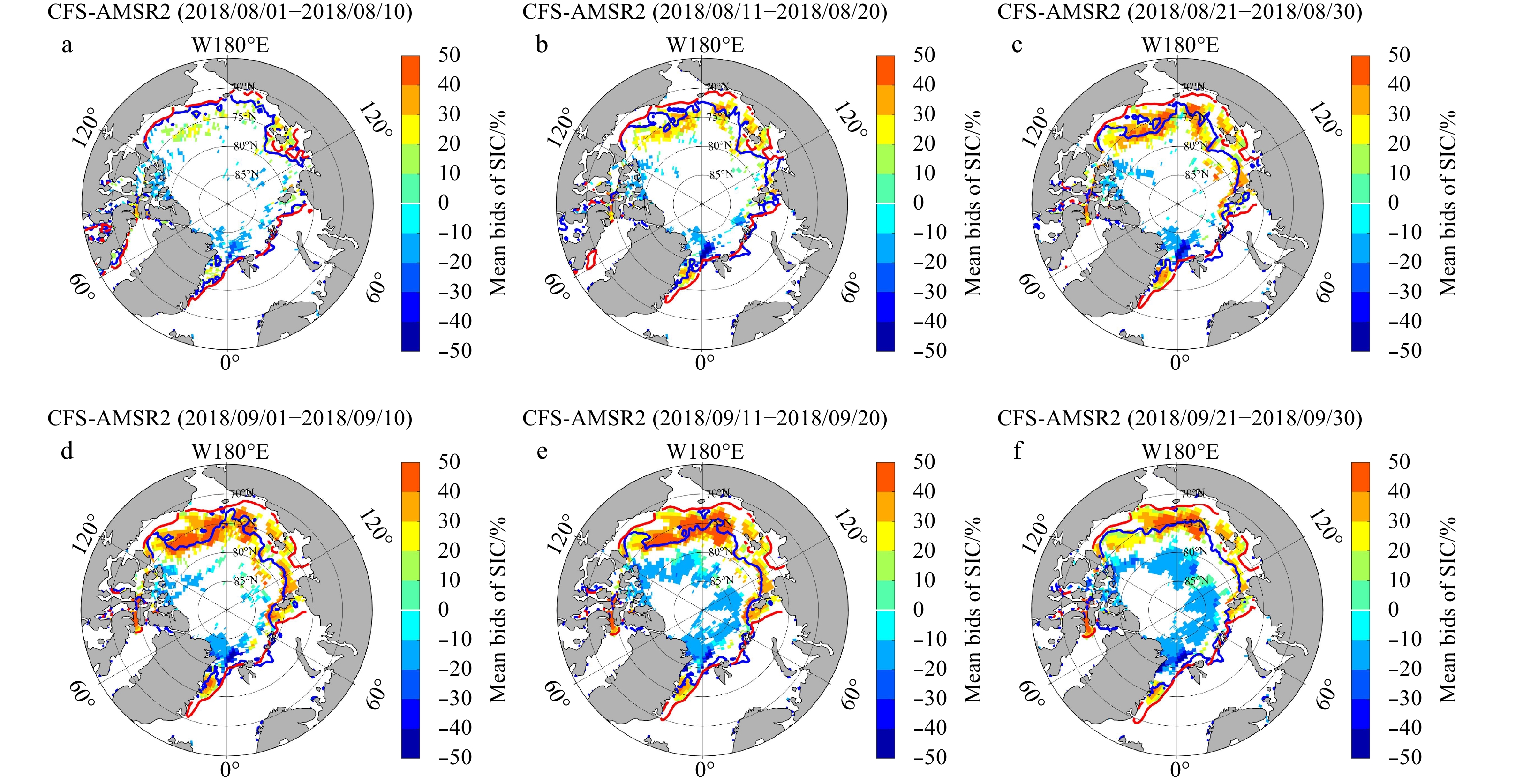
The CFS overestimated the SIC in the marginal ice zone, while it underestimated the SIC in the central area (Fig. 4). The positive mean bias increased from 26% in mid-August to 33% in late September, while the negative mean bias remained at a similar level of –16% during this period. The overestimation of SIE mainly occurred in the Beaufort Sea, Chukchi Sea, and New Siberian Sea, which gradually increased along with the increase in lead time (Fig. 4).
Figure
4.
The mean bias of the CFS SIC for different periods of 10 d in August and September. The blue lines and red lines represent the SIE from satellite observations and model predictions, respectively.
Two metrics were used to evaluate the role of bias correction on the predictions initialized on August 1, 2018. Root Mean Square Error (RMSE) was selected to reflect the overall SIC differences, while Integrated Ice Edge Error (IIEE) was used to assessing the disagreement of SIE between prediction and observation. It was expressed as sea ice extent sum of area where was covered by model forecasts, but not covered by satellite observations (overestimation by model), and area where was not covered by model forecasts, but covered by satellite observations (underestimation by model) (Goessling et al., 2016, 2018).
The bias correction was performed for the 60 d predictions from the FIOESM and CFS, which both was initialized on August 1, 2018. The comparison is illustrated in Figs 5 and 6, where the left column shows the raw results, the middle column shows the results with bias correction, and the right column shows the satellite observations.
Figure
5.
Arctic sea ice predictions by FIOESM and observations for the different periods of 10 d in August and September 2018. FIOESM prediction was initialized on August 1, 2018. The left column shows the raw results, the middle column shows the results with bias correction, and the right column shows the satellite observations.
Figure
6.
Arctic sea ice predictions by CFS and observations for the different periods of 10 d in August and September 2018. CFS prediction was initialized on August 1, 2018. The left column shows the raw results, the middle column shows the results with bias correction, and the right column shows the satellite observations.
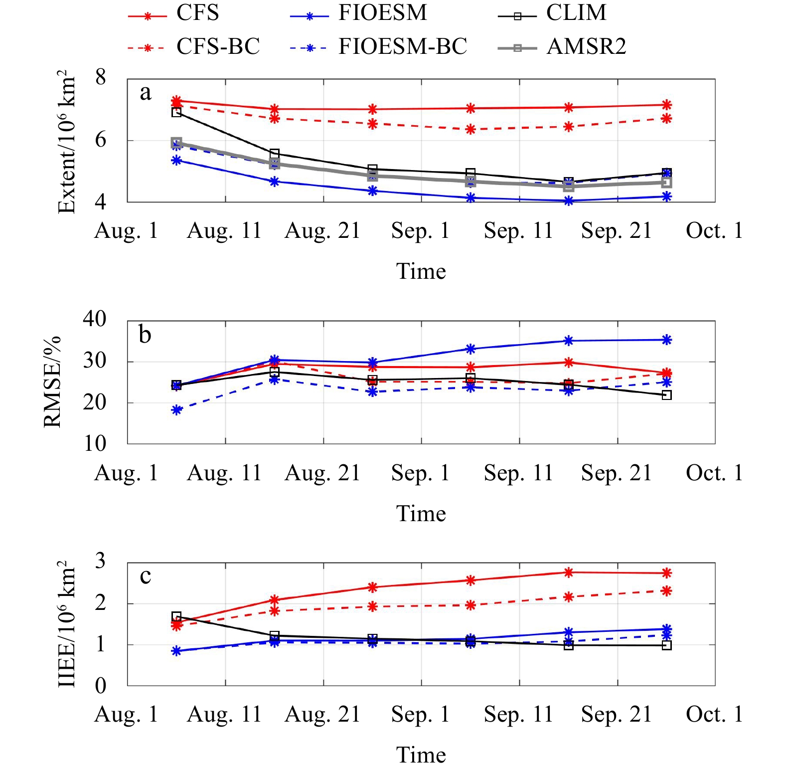
It is clear that the bias correction improved the SIC underestimation in the FIOESM raw prediction, where maximum SIC in the central Arctic (especially more northward than 85°N) was 80%–90% in the 10–50 d of predictions, which was not consistent with the 90%–100% high concentration obtained by observation. After bias correction, the SIC maximum was significantly improved, with a 27% reduction in the RMSE of SIC, from –33% to –24%. Similarly, the bias correction also had a positive effect on SIE, where IIEE showed a 10% improvement, decreasing from 1.21×10⁶ km2 to 1.09×10⁶ km2 (Fig. 7).
Figure
7.
Sea ice extent, RMSE and IIEE for different periods of 10 d for prediction initialized on August 1, 2018. The red and blue lines represented the results of CFS and FIOESM, respectively. The black lines represented CLIM benchmark forecasts and the gray lines represented AMSR2 observations.
The raw prediction from the CFS showed a reasonable SIC distribution in the central Arctic, but overestimated the marginal ice zone, especially in the Beaufort Sea and New Siberia Sea, where it was ice-free in the satellite products (Fig. 6). Bias correction significantly reduced the overestimation in the Beaufort Sea and New Siberia Sea. The RMSE of the overall SIC decreased by 7%, from 28% to 26%, while the IIEE of SIE underwent a 17% reduction, from 2.35×10⁶ km2 to 1.94×10⁶ km2 (Fig. 7). The increasing trend of the IIEE suggested that the disagreement with the SIE had a positive relationship with the model lead times.
Sea ice extent was calculated for quantifying the model capability to capture the minimum, and it is represented by the total area of the grid cell covered by a sea ice concentration larger than 15%. The capability of a model to project the time and amount of minimum sea ice extent is thought to be key performance index for the Arctic. As shown by the gray lines in Fig. 7, the observed minimum sea ice extent occurred in the middle of September, with an amount of 4.51×10⁶ km2. The CFS largely overestimated the sea ice extent and failed to capture the time of minimum sea ice extent, which was estimated to be late August before bias correction and early September after bias correction. The FIOESM predicted a reasonable amount of variation in sea ice extent in August and September and perfectly capture the time of minimum sea ice extent, especially after bias correction, when the amount was predicted to be 4.62×10⁶ km2. These results were consistent with the satellite observations (Table 2).
Table
2.
Statistics for the 60 d projections initialized on August 1, 2018
For sea ice extent, benchmark forecasts of CLIM outperformed both CFS raw data and CFS-BC data, as shown in Fig. 7a. FIOESM-BC data matched well with sea ice extent observations and outperformed CLIM for all the periods. In term of RMSE, the raw products of FIOESM and CFS were only comparable in the period of first ten days, which was consistent with the comparison results of S2S models in Zampieri et al. (2018), while FIOESM performed better with bias correction (Fig. 7b). Regarding IIEE, it is obvious that CFS overestimation lasted for all the periods, while FIOESM raw data and FIOESM-BC data was close to CLIM benchmark forecasts from the second to the sixth 10 d (Fig. 7c).
5.
Discussion
5.1
Initialization on different dates
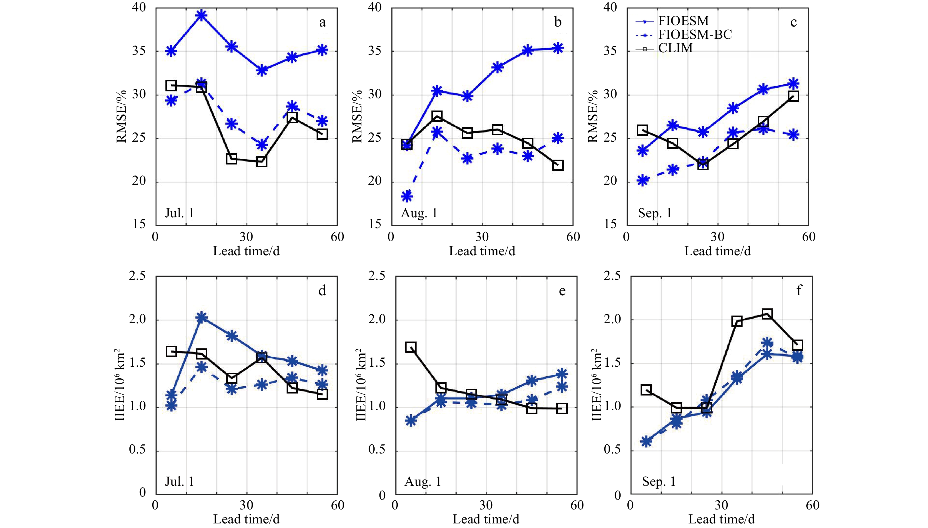
The prediction initialized on different dates was analyzed here, to assess the effectiveness of the bias correction method during the entire summer season. Both RMSE and IIEE decreased obviously when the initialization dates forwarded from July 1 to August 1, then to September 1 (Fig. 8). The reason may be related to the fact that pack sea ice covered most of the marginal sea in July with relative small concentration, while it retreated to the high latitude area with very high concentration. The low concentration marginal area was usually the main bias resource for climate models (Shu et al., 2015b; Director et al., 2017). The improvement introduced by bias correction for both RMSE and IIEE was smaller in September, when the ice extent reaches its minimum. FIOESM-BC forecasts usually performed better than CLIM benchmark forecasts at the early stage, but not so at the later stage.
Figure
8.
RMSE and IIEE for different lead time from FIOESM, initialized on July 1, August 1, and September 1 of 2018. The blue solid and dashed lines represent results before and after bias correction, respectively. The black lines represented CLIM benchmark forecasts.
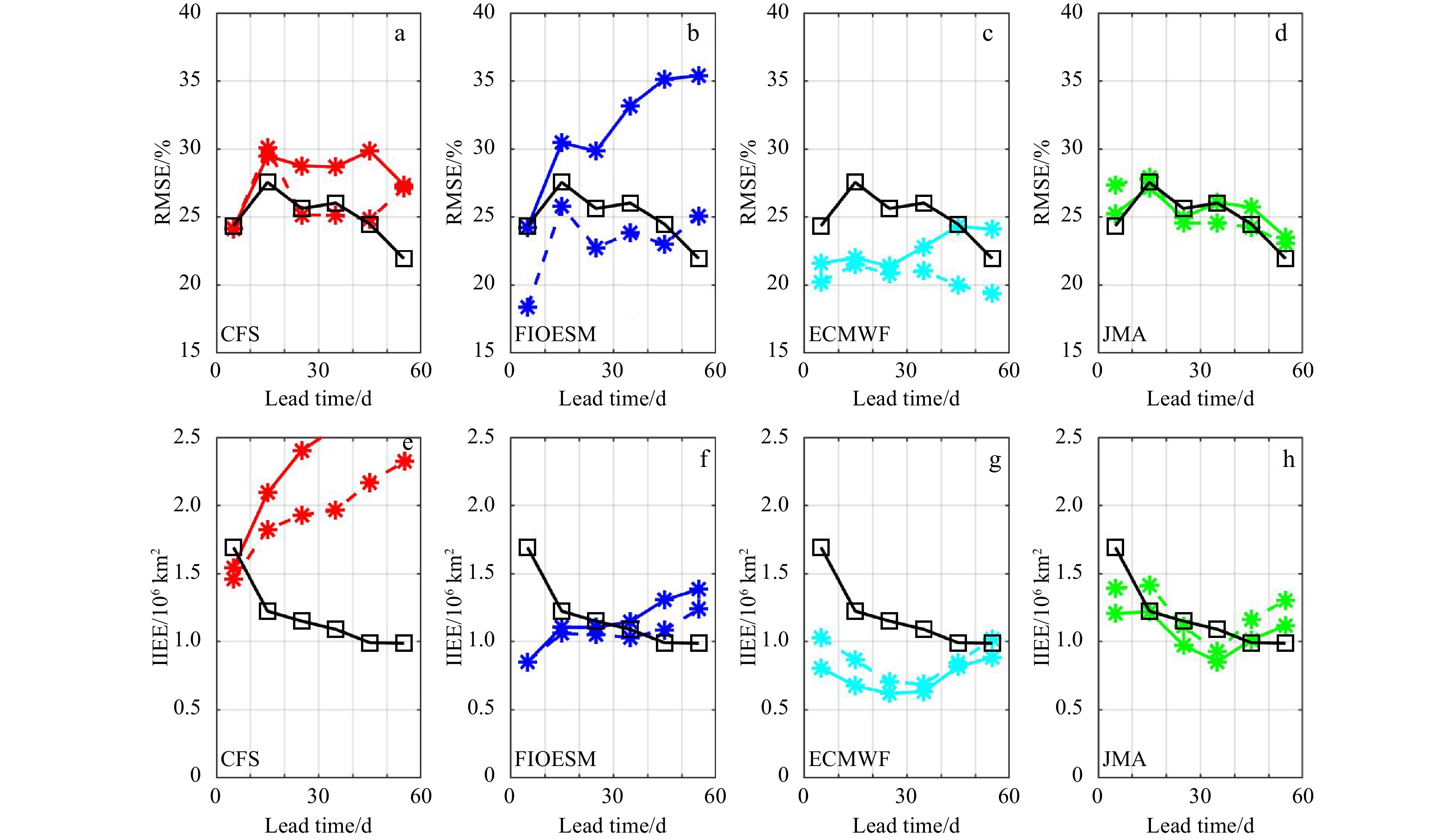
ECMWF and JMA forecasts were added to the comparison with CFS and FIOESM to further investigate the influence of bias correction on different models. The results in Fig. 9 suggested that ECMWF performed the best for both RMSE and IIEE. Bias correction improved slightly for RMSE, but IIEE became worse. JMA was close to CLIM benchmark forecasts with little effect from bias correction. The comparison indicated that the role of bias correction acted more positively when the bias itself was larger, for example RMSE of FIOESM and IIEE of CFS. After all, the improvement with bias correction was not consistent for different models, which may be related to the spatial and temporal features of bias distribution of models.
Figure
9.
RMSE and IIEE for different models, initialized on August 1, 2018. The solid and dashed lines represent results before and after bias correction, respectively. The black lines represented CLIM benchmark forecasts.
Scientific exploration and commercial shipping activities in the Arctic have become frequent in recent years due to the rapid decline in Arctic sea ice. By the summer of 2018, China had conducted nine national research expeditions and 22 commercial shipping voyages in this region. At present, subseasonal projection of SIC and extent using dynamic models is the main approach employed by stockholders to estimate future sea ice conditions. However, physical uncertainties in climate models introduce large biases to subseasonal predictions, and therefore bias correction technology is essential, especially when the predictions are used for practical sea ice services for icebreakers or commercial ships.
In this study, we proposed one method for bias correction and performed in raw prediction products from two climate models, FIOESM and CFS, to yield bias-corrected productions. Both models were initialized on August 1, 2018, and run for two months, as part of the official sea ice service for the ninth CHINARE and COSCO Northeast Passage voyages during the summer of 2018. The 60 d predictions were analyzed by comparing the RMSE (of SIC) and IIEE (of SIE) of the raw products and the bias-corrected products. The raw predictions from the FIOESM showed an overall SIC underestimation in the ice-covered region, with a mean bias of SIC up to approximately 30%. Bias correction brought a 27% improvement in the RMSE of SIC and a 10% improvement in the IIEE of SIE. By contrast, for CFS, the SIE overestimation in the marginal ice zone was its domain features. Bias correction introduced a 7% improvement in the RMSE of SIC and a 17% improvement in the IIEE of SIE. In brief, the bias correction performed in this study largely improved the SIC underestimation of FIOESM and SIE overestimation of CFS. In terms of sea ice extent, FIOESM captured the seasonal variation and a reasonable time and amount of minimum sea ice extent in mid-September; while CFS failed to accurately project both the time and amount of minimum sea ice extent.
The analysis of different initialization dates showed that the influence of bias correction on RMSE and IIEE improvement was obvious, especially for the predictions with large bias. The comparison with S2S results suggested that the method of bias correction was model-dependent, with large improvement on models with large bias. Overall, the proposed bias correction methodology in this paper improved the forecasts, especially if large biases are present.
Subseasonal sea ice projection in summer is critically important for Arctic cruise planning. However, because of the limitations of model capabilities, there is a large gap between the raw prediction products and actual conditions. The combination of bias correction methodologies with climate model in this study has been demonstrated as an effective tool for increasing the accuracy of predictions along with further developments and improvements in physical parameterization and data assimilation for climate models. Hopefully, improvements in model physics and bias correction techniques will lead to better predictive skills in the future.
Blanchard-Wrigglesworth E, Barthelemy A, Chevallier M, et al. 2017. Multi-model seasonal forecast of Arctic sea-ice: forecast uncertainty at pan-Arctic and regional scales. Climate Dynamics, 49(4): 1399–1410. doi: 10.1007/s00382-016-3388-9
[2]
Blanchard-Wrigglesworth E, Cullather R I, Wang Wanqiu, et al. 2015. Model forecast skill and sensitivity to initial conditions in the seasonal sea ice outlook. Geophysical Research Letters, 42(19): 8042–8048. doi: 10.1002/2015GL065860
[3]
Chen Hui, Yin Xunqiang, Bao Ying, et al. 2016. Ocean satellite data assimilation experiments in FIO-ESM using ensemble adjustment Kalman filter. Science China Earth Sciences, 59(3): 484–494. doi: 10.1007/s11430-015-5187-2
[4]
Comiso J C, Parkinson C L, Gersten R, et al. 2008. Accelerated decline in the Arctic sea ice cover. Geophysical Research Letter, 35(1): L01703
[5]
Director H M, Raftery A E, Bitz C M. 2017. Improved sea ice forecasting through spatiotemporal bias correction. Journal of Climate, 30(23): 9493–9510. doi: 10.1175/JCLI-D-17-0185.1
[6]
Ek M B, Mitchell K E, Lin Y, et al. 2003. Implementation of Noah land surface model advances in the National Centers for Environmental Prediction operational mesoscale Eta model. Journal of Geophysical Research: Atmosphere, 108(D22): 8851
[7]
Goessling H F, Jung T. 2018. A probabilistic verification score for contours: methodology and application to Arctic ice-edge forecasts. Quarterly Journal of the Royal Meteorological Society, 144(712): 735–743. doi: 10.1002/qj.3242
[8]
Goessling H F, Tietsche S, Day J J, et al. 2016. Predictability of the Arctic sea ice edge. Geophysical Research Letters, 43(4): 1642–1650. doi: 10.1002/2015GL067232
[9]
Griffies S M, Harrison M J, Pacanowski R C, et al. 2004. A technical guide to MOM4. GFDL Ocean Group Technical Report No.5. Princeton, US: Geophysical Fluid Dynamics Laboratory, NOAA
[10]
Hawkins E, Osborne T M, Ho C K, et al. 2013. Calibration and bias correction of climate projections for crop modelling: an idealised case study over Europe. Agricultural and Forest Meteorology, 170: 19–31. doi: 10.1016/j.agrformet.2012.04.007
Hunke E C, Dukowicz J K. 1997. An elastic-viscous-plastic model for sea ice dynamics. Journal of Physical Oceanography, 27(9): 1849–1867. doi: 10.1175/1520-0485(1997)027<1849:AEVPMF>2.0.CO;2
[13]
Huntingford C, Lambert H F, Gash J H C, et al. 2005. Aspects of climate change prediction relevant to crop productivity. Philosophical Transactions of the Royal Society B: Biological Sciences, 360(1463): 1999–2009. doi: 10.1098/rstb.2005.1748
[14]
Ines A V M, Hansen J W. 2006. Bias correction of daily GCM rainfall for crop simulation studies. Agricultural and Forest Meteorology, 138(1–4): 44–53
[15]
Kwok R, Cunningham G F, Wensnahan M, et al. 2009. Thinning and volume loss of the Arctic Ocean sea ice cover: 2003–2008. Journal of Geophysical Research: Oceans, 114(C7): C07005
[16]
Liu Jiping, Chen Zhiqiang, Hu Yongyun, et al. 2019. Towards reliable Arctic sea ice prediction using multivariate data assimilation. Science Bulletin, 64(1): 63–72. doi: 10.1016/j.scib.2018.11.018
[17]
Markus T, Stroeve J C, Miller J. 2009. Recent changes in Arctic sea ice melt onset, freezeup, and melt season length. Journal of Geophysical Research: Oceans, 114(C12): C12024. doi: 10.1029/2009JC005436
[18]
Meehl G A, Goddard L, Boer G, et al. 2014. Decadal climate prediction: an update from the trenches. Bulletin of the American Meteorological Society, 95(2): 243–267. doi: 10.1175/BAMS-D-12-00241.1
[19]
Nghiem S V, Rigor I G, Perovich D K, et al. 2007. Rapid reduction of Arctic perennial sea ice. Geophysical Research Letters, 34(19): L19504. doi: 10.1029/2007GL031138
[20]
Qiao Fangli, Song Zhenya, Bao Ying, et al. 2013. Development and evaluation of an Earth System Model with surface gravity waves. Journal of Geophysical Research: Oceans, 118(9): 4514–4524. doi: 10.1002/jgrc.20327
[21]
Qiao Fangli, Yuan Yeli, Yang Yongzeng, et al. 2004. Wave-induced mixing in the upper ocean: distribution and application to a global ocean circulation model. Geophysical Research Letters, 31(11): L11303
[22]
Saha S, Moorthi S, Wu Xingren, et al. 2010. The NCEP climate forecast system reanalysis. Bulletin of the American Meteorological Society, 91(8): 1015–1057. doi: 10.1175/2010BAMS3001.1
[23]
Saha S, Moorthi S, Wu Xingren, et al. 2014. The NCEP climate forecast system version 2. Journal of Climate, 27(6): 2185–2208. doi: 10.1175/JCLI-D-12-00823.1
[24]
Shu Qi, Qiao Fangli, Bao Ying, et al. 2015a. Assessment of Arctic sea ice simulation by FIO-ESM based on data assimilation experiment. Haiyang Xuebao (in Chinese), 37(11): 33–40
[25]
Shu Qi, Song Zhenya, Qiao Fangli. 2015b. Assessment of sea ice simulations in the CMIP5 models. The Cryosphere, 9(1): 399–409. doi: 10.5194/tc-9-399-2015
[26]
Spreen G, Kaleschke L, Heygster G. 2008. Sea ice remote sensing using AMSR-E 89-GHz channels. Journal of Geophysical Research: Oceans, 113(C2): C02S03
[27]
Stroeve J, Hamilton L C, Bitz C M, et al. 2014. Predicting September sea ice: ensemble skill of the SEARCH sea ice outlook 2008–2013. Geophysical Research Letters, 41(7): 2411–2418. doi: 10.1002/2014GL059388
[28]
Stroeve J C, Serreze M C, Holland M M, et al. 2012. The Arctic’s rapidly shrinking sea ice cover: a research synthesis. Climatic Change, 110(3): 1005–1027
[29]
Vitart F, Ardilouze A, Bonet A, et al. 2017. The Subseasonal to Seasonal (S2S) prediction project database. Bulletin of the American Meteorological Society, 98: 163–173. doi: 10.1175/BAMS-D-16-0017.1
[30]
Wayand N E, Bitz C M, Blanchard-Wrigglesworth E. 2019. A year-round subseasonal-to-seasonal sea ice prediction portal. Geophysical Research Letters, 46(6): 3298–3307. doi: 10.1029/2018GL081565
Zampieri L, Goessling H F, Jung T. 2018. Bright prospects for arctic sea ice prediction on subseasonal time scales. Geophysical Research Letters, 45(18): 9731–9738. doi: 10.1029/2018GL079394
[33]
Zampieri L, Goessling H F, Jung T. 2019. Predictability of Antarctic sea ice edge on subseasonal time scales. Geophysical Research Letters, 46(16): 9719–9727. doi: 10.1029/2019GL084096
[34]
Zhao Jiechen, Zhou Xiang, Sun Xiaoyu, et al. 2017. The inter comparison and assessment of satellite sea-ice concentration datasets from the arctic. Journal of Remote Sensing (in Chinese), 21(3): 351–364
Cyril Palerme, Thomas Lavergne, Jozef Rusin, et al. Improving short-term sea ice concentration forecasts using deep learning. The Cryosphere, 2024, 18(4): 2161. doi:10.5194/tc-18-2161-2024
2.
Shijin Yuan, Shichen Zhu, Xiaodan Luo, et al. A deep learning-based bias correction model for Arctic sea ice concentration towards MITgcm. Ocean Modelling, 2024, 188: 102326. doi:10.1016/j.ocemod.2024.102326
3.
Chungkham Thombson, Rajkumar Kamaljit Singh, Sandip Rashmikant Oza, et al. Estimation of Sea Ice Concentration in the Arctic Using SARAL/AltiKa Data. IEEE Transactions on Geoscience and Remote Sensing, 2023, 61: 1. doi:10.1109/TGRS.2023.3328786
4.
Peter A. Bieniek, Hajo Eicken, Meibing Jin, et al. Seasonal forecasting of landfast ice in Foggy Island Bay, Alaska in support of ice road operations. Cold Regions Science and Technology, 2022, 201: 103618. doi:10.1016/j.coldregions.2022.103618
5.
Arlan Dirkson, Bertrand Denis, William J. Merryfield, et al. Calibration of subseasonal sea‐ice forecasts using ensemble model output statistics and observational uncertainty. Quarterly Journal of the Royal Meteorological Society, 2022, 148(747): 2717. doi:10.1002/qj.4332
6.
Ruibo Lei, Zexun Wei. Exploring the Arctic Ocean under Arctic amplification. Acta Oceanologica Sinica, 2020, 39(9): 1. doi:10.1007/s13131-020-1642-9
Figure 1. The Route of icebreaker Xuelong (solid black line) and COSCO commercial voyages (dashed line in different colors) during summer 2018. The sea ice concentration of August 1, 2018 was illustrated. The date inside brackets after the ship names represented the period they sailed in Arctic.
Figure 2. Schematic of the bias correction methodology. Bias correction uses raw model output for the future period, and corrects it using the bias ($ {\Delta }_{\mathrm{R}\mathrm{E}\mathrm{F}} $) between historical reference data from the model and observations. $ {O}_{\mathrm{R}\mathrm{E}\mathrm{F}} $ means observations during the historical reference period, $ {SIC}_{\mathrm{R}\mathrm{E}\mathrm{F}} $ means model output from the historical reference period, $ {SIC}_{\mathrm{R}\mathrm{A}\mathrm{W}} $ means raw model output for the prediction period, and $ {SIC}_{\mathrm{B}\mathrm{C}} $ means bias-corrected output.
Figure 3. The mean bias of the FIOESM SIC for different periods of 10 d in August and September. The blue lines and red lines represent the SIE from satellite observations and model predictions, respectively.
Figure 4. The mean bias of the CFS SIC for different periods of 10 d in August and September. The blue lines and red lines represent the SIE from satellite observations and model predictions, respectively.
Figure 5. Arctic sea ice predictions by FIOESM and observations for the different periods of 10 d in August and September 2018. FIOESM prediction was initialized on August 1, 2018. The left column shows the raw results, the middle column shows the results with bias correction, and the right column shows the satellite observations.
Figure 6. Arctic sea ice predictions by CFS and observations for the different periods of 10 d in August and September 2018. CFS prediction was initialized on August 1, 2018. The left column shows the raw results, the middle column shows the results with bias correction, and the right column shows the satellite observations.
Figure 7. Sea ice extent, RMSE and IIEE for different periods of 10 d for prediction initialized on August 1, 2018. The red and blue lines represented the results of CFS and FIOESM, respectively. The black lines represented CLIM benchmark forecasts and the gray lines represented AMSR2 observations.
Figure 8. RMSE and IIEE for different lead time from FIOESM, initialized on July 1, August 1, and September 1 of 2018. The blue solid and dashed lines represent results before and after bias correction, respectively. The black lines represented CLIM benchmark forecasts.
Figure 9. RMSE and IIEE for different models, initialized on August 1, 2018. The solid and dashed lines represent results before and after bias correction, respectively. The black lines represented CLIM benchmark forecasts.


 DownLoad:
 DownLoad:


 DownLoad: