Tian Ma, Xuhua Cheng, Yiquan Qi, Jiajia Chen. Interannual variability in the barrier layer and forcing mechanism in the eastern equatorial Indian Ocean and Bay of Bengal[J]. Acta Oceanologica Sinica, 2020, 39(7): 19-31. doi: 10.1007/s13131-020-1575-3
Citation:
Tian Ma, Xuhua Cheng, Yiquan Qi, Jiajia Chen. Interannual variability in the barrier layer and forcing mechanism in the eastern equatorial Indian Ocean and Bay of Bengal[J]. Acta Oceanologica Sinica, 2020, 39(7): 19-31. doi: 10.1007/s13131-020-1575-3
Tian Ma, Xuhua Cheng, Yiquan Qi, Jiajia Chen. Interannual variability in the barrier layer and forcing mechanism in the eastern equatorial Indian Ocean and Bay of Bengal[J]. Acta Oceanologica Sinica, 2020, 39(7): 19-31. doi: 10.1007/s13131-020-1575-3
Citation:
Tian Ma, Xuhua Cheng, Yiquan Qi, Jiajia Chen. Interannual variability in the barrier layer and forcing mechanism in the eastern equatorial Indian Ocean and Bay of Bengal[J]. Acta Oceanologica Sinica, 2020, 39(7): 19-31. doi: 10.1007/s13131-020-1575-3
Key Laboratory of Marine Hazards Forecasting, Ministry of Natural Resources, Hohai University, Nanjing 210098, China
2.
College of Oceanography, Hohai University, Nanjing 210098, China
3.
Southern Marine Science and Engineering Guangdong Laboratory (Zhuhai), Zhuhai 519000, China
Funds:
The National Key R&D Program of China under contract No. 2018YFA0605702; the National Natural Science Foundation of China under contract Nos 41522601, 41876002 and 41876224; the Fundamental Research Funds for the Central Universities under contract Nos 2017B04714 and 2017B4114.
Interannual variability (IAV) in the barrier layer thickness (BLT) and forcing mechanisms in the eastern equatorial Indian Ocean (EEIO) and Bay of Bengal (BoB) are examined using monthly Argo data sets during 2002–2017. The BLT during November–January (NDJ) in the EEIO shows strong IAV, which is associated with the Indian Ocean dipole mode (IOD), with the IOD leading the BLT by two months. During the negative IOD phase, the westerly wind anomalies driving the downwelling Kelvin waves increase the isothermal layer depth (ILD). Moreover, the variability in the mixed layer depth (MLD) is complex. Affected by the Wyrtki jet, the MLD presents negative anomalies west of 85°E and strong positive anomalies between 85°E and 93°E. Therefore, the BLT shows positive anomalies except between 86°E and 92°E in the EEIO. Additionally, the IAV in the BLT during December–February (DJF) in the BoB is also investigated. In the eastern and northeastern BoB, the IAV in the BLT is remotely forced by equatorial zonal wind stress anomalies associated with the El Niño-Southern Oscillation (ENSO). In the western BoB, the regional surface wind forcing-related ENSO modulates the BLT variations.
The eastern equatorial Indian Ocean (EEIO) and Bay of Bengal (BoB), as parts of the Indo-Pacific warm pool, play a key role in regulating the global climate by air-sea interaction (Oppo et al., 2009). The sea surface temperature (SST) of these areas is close to or greater than 28°C except during winter, so slight SST variations lead to a strong atmospheric circulation responses, which have a significant impact on the climate and monsoon precipitation in the surrounding areas (Palmer and Mansfield, 1984; Li et al., 2001; Shankar et al., 2007; Jiang and Li, 2011).
The BoB is one of the lowest salinity ocean basins in the world due to the large amount of freshwater runoff from hinterland rivers around the BoB and the abundant rainfall during the summer monsoon (Varkey et al., 1996). This injection of fresh water significantly strengthens salinity stratification in the upper layer, providing the conditions necessary for the formation of a barrier layer (BL) sandwiched between the mixing layer (ML) and the isothermal layer (IL) (Vinayachandran et al., 2002). The BL plays the role of a heat barrier in the vertical heat exchange between the ML and the thermocline and can help explain the warm SSTs (>28ºC) (Godfrey and Lindstrom, 1989; Shenoi et al., 2002). Therefore, study of the variations in the BL is particularly valuable for understanding the air-sea interaction, especially during the summer monsoon.
Lindstrom et al. (1987) first noticed that there is an obvious layer between the ML bottom and IL bottom, in which the temperature is uniform and the salinity increases rapidly with depth. Later, Lukas and Lindstrom (1991) introduced the barrier layer concept to describe this physical phenomenon. Since then, a number of studies have examined its formation mechanisms, spatial distribution and effects on air-sea interaction in the equatorial Pacific Ocean, the equatorial Atlantic Ocean and the equatorial Indian Ocean (EIO) (Sprintall and Tomczak, 1992; You, 1995; 1998; Vialard et al., 1998; Qu and Meyers, 2005; Maes et al., 2005; Breugem et al., 2008; De Boyer Montegut et al., 2007). The seasonal evolution of the BL in the EEIO has been investigated. The barrier layer thickness (BLT) in the EEIO reaches its annual maximum in November and is regulated by the Wyrtki jet and surface circulation (Masson et al., 2002; Qiu et al., 2012). In the BoB, the BLT reaches its maximum in winter, and the surface circulation and the redistribution of low-salinity waters have a dominant impact on the observed BL distribution. In addition, the BL is also modulated by Ekman pumping and Rossby waves radiated by the coastal Kelvin waves (Thadathil et al., 2007). The interplay between rainfall and surface current also play an important role for forming thick BL (Agarwal et al., 2012). In winter, the BL always contains inversions in the vertical temperature profiles, which means that the subsurface temperature is higher than the surface temperature (Thadathil et al., 2002; Rao and Sivakumar, 2003; Thompson et al., 2006; Girishkumar et al., 2013; Thangaprakash et al., 2016).
In the past 10 years, with the increase in observational data, numerous studies have investigated the intraseasonal variability to interannual variability (IAV) in the BLT in the EEIO and BoB. In the southern BoB, the intraseasonal variability in the BLT is mainly regulated by the vertical movement of the isothermal layer depth (ILD), which is modulated primarily by vertical stretching of the upper water column associated with westward propagating Rossby waves remotely forced by intraseasonal surface wind in the EIO (Girishkumar et al., 2011). Previous studies also noted on the IAV in BLT co-propagates with Kelvin and Rossby waves during IOD years in the EIO (Chowdary et al., 2009; Cai et al., 2009). In the EEIO, the IAV in the BL is closely related to the Indian Ocean dipole (IOD), with the IOD leading the BL by one month. During the positive (negative) IOD season, equatorial easterly (westerly) wind anomalies induce upwelling (downwelling) Kelvin waves, which raise (deepen) the ILD, leading to the thinning (thickening) of BL (Qiu et al., 2012). However, due to the lack of long-term continuous observation data, this study only selected typical IOD years for discussion. Moreover, this study analyzes the IAV in the BLT during the mature phase of the IOD rather than the BLT. Furthermore, the upwelling (downwelling) Kelvin waves propagate eastward, reach the western coast of Sumatra, and reflect to propagate around the BoB as coastally trapped waves; these waves radiate Rossby waves and control the IAV in the BLT in the BoB (Cyriac et al., 2016; Kumari et al., 2018). Valsala et al. (2018) studied the IAV in the BLT in the BoB using observation data and model data for the period of 1995 to 2009 and showed that the BL IAV is predominantly controlled by El Niño-Southern Oscillation (ENSO)-related precipitation forcing. Yuan and Su (2019) found that both IOD and ENSO could impact the variability in BLT in EIO by influencing thermocline and sea surface salinity (SSS) using Simple Ocean Data Assimilation (SODA) data. In addition, Pang et al. (2019) analyzed the decadal variability in BLT and its forcing mechanisms in the BoB by using SODA dataset, and indicated that Pacific Decadal Oscillation (PDO) can indirectly modulate the decadal variations in BLT by exerting an influence on the Walker circulation. Although these studies attempt to describe the IAV or even decadal variability in the BLT, it is difficult to accurately calculate the BLT because the vertical stratification is not well reproduced in models (Fousiya et al., 2016).
The main aim of the present study is to investigate the IAV in the BLT during November–February in the EEIO and BoB. We consider the BLT during November–February because of its strong IAV and the occurrence of the temperature inversion during the winter, and the results provide a better understanding of the thermal and dynamic processes in the upper ocean from year to year. Since 2002, there have been more than 50 000 available observed profiles from Argo buoys collected in the EEIO and BoB. These floats offer a tremendous opportunity for us to study the upper ocean dynamic processes on interannual timescales.
2.
Materials and methods
2.1
Data
In this study, the temperature and salinity data provided by gridded monthly Argo products (ISAS15) reconstructed by the Laboratoire d’Océanographie Physique et Spatiale (LOPS) are used to calculate the ILD, mixed layer depth (MLD) and BLT (Gaillard et al., 2016). The products have a spatial resolution of a 0.5° regular grid from 2002 to 2015. Vertically, from the surface to 10 m depth, data are obtained at discrete depth intervals of 1 m, 3 m, 5 m, and 10 m. From 10–100 m, the resolution is 5 m; from 100–800 m, the resolution is 10 m; and from 800–2 000 m, the resolution is 20 m (http://www.umr-lops.fr/). In addition, the temperature and salinity grid data processed by the same algorithm are provided by the Copernicus Marine Environment Monitoring Service (CMEMS) from 2016 to 2017 with the same spatiotemporal resolution in the upper ocean.
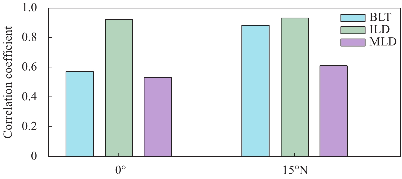
The RAMA buoys at 0°N, 90°E and 15°N, 90°E provides daily time series of temperatures at depths of 1, 10, 13, 20, 40, 60, 80, 100, 120, 140, 180, 300, and 500 m and of salinity at depths of 1, 5, 10, 20, 40, 60, 100, and 140 m (McPhaden et al., 2009). In some time periods, the buoy observations were seriously disrupted by natural conditions, and the data are missing to some extent. This paper examined only the available data. To verify the reliability of the Argo grid data, we compared the monthly average RAMA data with the Argo grid data, as shown in Fig. 1. At 0, 90°E, the correlation coefficients for BLT, ILD and MLD are 0.57, 0.92 and 0.53, respectively, all of which pass the significance test of 95%. The slightly lower correlation coefficients for MLD and BLT are mainly due to the slight deviation in the vertical salinity profiles in the Argo data and the relatively short time series of continuous observations by RAMA buoys from September 2009 to May 2013. At 15°N, 90°E, the time series is longer, from January 2008 to December 2015. The correlation coefficients for BLT, ILD and MLD are 0.88, 0.93 and 0.61, respectively. In general, the Argo grid data represent a very good description of the vertical temperature distribution but do not provide as good of a description of the vertical salinity distribution; however, this limitation has no significant influence on calculating the BLT.
Figure
1.
Correlation coefficients for BLT, ILD and MLD between Argo grid data and RAMA data at 0°, 90°E and 15°N, 90°E. BLT: barrier layer thickness; ILD: isothermal layer depth; MLD: mixed layer depth.
The monthly surface wind, evaporation and precipitation data with a resolution of 0.25°×0.25° from 2002 to 2017 are obtained from the ERA-Interim reanalysis provided by the European Centre for Medium-Range Weather Forecasts (ECMWF) (Dee et al., 2011).
The monthly SST anomalies are computed from the optimum interpolation sea surface temperature (OISST) data sets provided by the National Oceanic and Atmospheric Administration (NOAA), which are used to compute the IOD index. The Niño 3.4 index is provided by the Climate Prediction Center (CPC) of NOAA.
2.2
Method
In this study, the ILD is defined as the depth at which the temperature is 0.6°C lower than that at 10 m depth. The MLD is defined as the depth at which the density increases from that at the surface by an amount equal to the increase in density caused by a 0.6°C decrease in temperature (Kara et al., 2000; Qu and Meyers, 2005). The BLT is then defined as the difference between the depths of the IL and the ML. According to this standard, the MLD considers the influence of both temperature and salinity. When the salinity in the IL has a positive downward salinity gradient, the ML will be shallower than the IL. In addition, following Girishkumar et al. (2013), temperature inversions are defined as when the temperature at depth is greater than the temperature at 10 m depth by 0.1°C.
According to the ECMWF, the wind stress curl is defined as:
where $ {\rm {Curl}}_{z} $ is the wind stress curl, $ {\tau }_{x} $ and $ {\tau }_{y} $ are the wind stress in the $ x $ and $ y $ directions, respectively. The $ \tau $ is defined as follows:
$$
\tau ={\rho }_{a}{C}_{D}{U}_{10}^{2},
$$
(2)
where $ {\rho }_{a} $ is density of air, its value is 1.3 kg/m3, and $ {C}_{D} $ is the drag coefficient, which is calculated by referring to Yelland and Taylor (1996). Additionally, $ {U}_{10} $ is the wind speed at 10 m on the sea surface.
3.
Seasonal cycle of the BLT
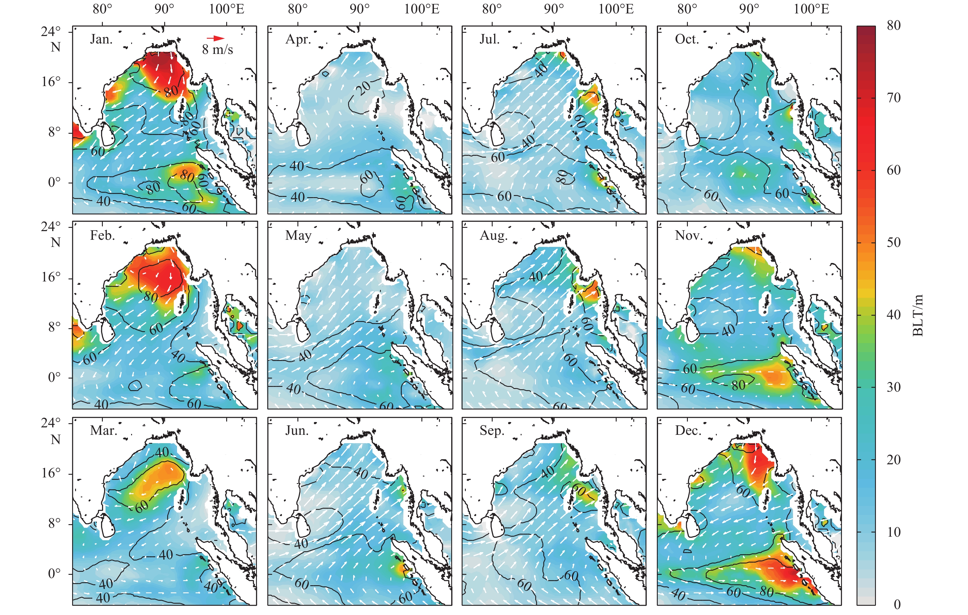
Previous studies have done lots of work of the seasonal cycle of the BLT and its formation mechanism in the EEIO and the BoB (Masson et al., 2002; Thadathil et al., 2007; Agarwal et al., 2012; Qiu et al., 2012; Kumari et al., 2018; Shee et al., 2019). Based on the data with higher spatial and temporal resolution, now we expect to reveal more detailed features about the seasonal cycle of the BLT on the basis of previous frameworks. The monthly mean climatology of the BLT in the EEIO and BoB for the period 2002–2017 is shown in Fig. 2. In the EEIO, the results showed that a thick BL (of more than 30 m) is observed near the western coast of Sumatra Island from April to June and from October to December and that the BL then gradually deepens and extends to the west. The BLT attains its annual maximum (more than 60 m) during December. From April to June and from October to December, driven by westerly winds, the Wyrtki jet (Wyrtki, 1973) carries high-salinity water from the Arabian Sea to the EEIO, forming salinity stratification with fresh water on the surface. Moreover, the downwelling Kelvin waves, which are also driven by westerly winds, deepen the IL (Rao et al., 2010). Then, the IL separates from the ML due to the salinity stratification, and a thicker BL forms. The stronger westerly winds in autumn drive the stronger downwelling Kelvin waves, and decreased SST occur at the surface; hence, the IL is deeper, and the BL reaches its annual maximum. From January to March and July to September, the easterly winds drive upwelling Kelvin waves, which make the IL and ML gradually shallower, and the BL gradually thinner. The seasonal cycle of the BLT and its formation mechanism presented in this study is similar to that of Masson et al. (2002) and Qiu et al. (2012). However, previous works suggested that the BLT reaches its annual maximum during November, but in the present study, the annual BLT maximum is observed in December.
Figure
2.
Monthly mean climatology of Argo BLT (shading, m), ILD (contours, m) and ECMWF surface winds (vectors, m/s). BLT: barrier layer thickness; ILD: isothermal layer depth.
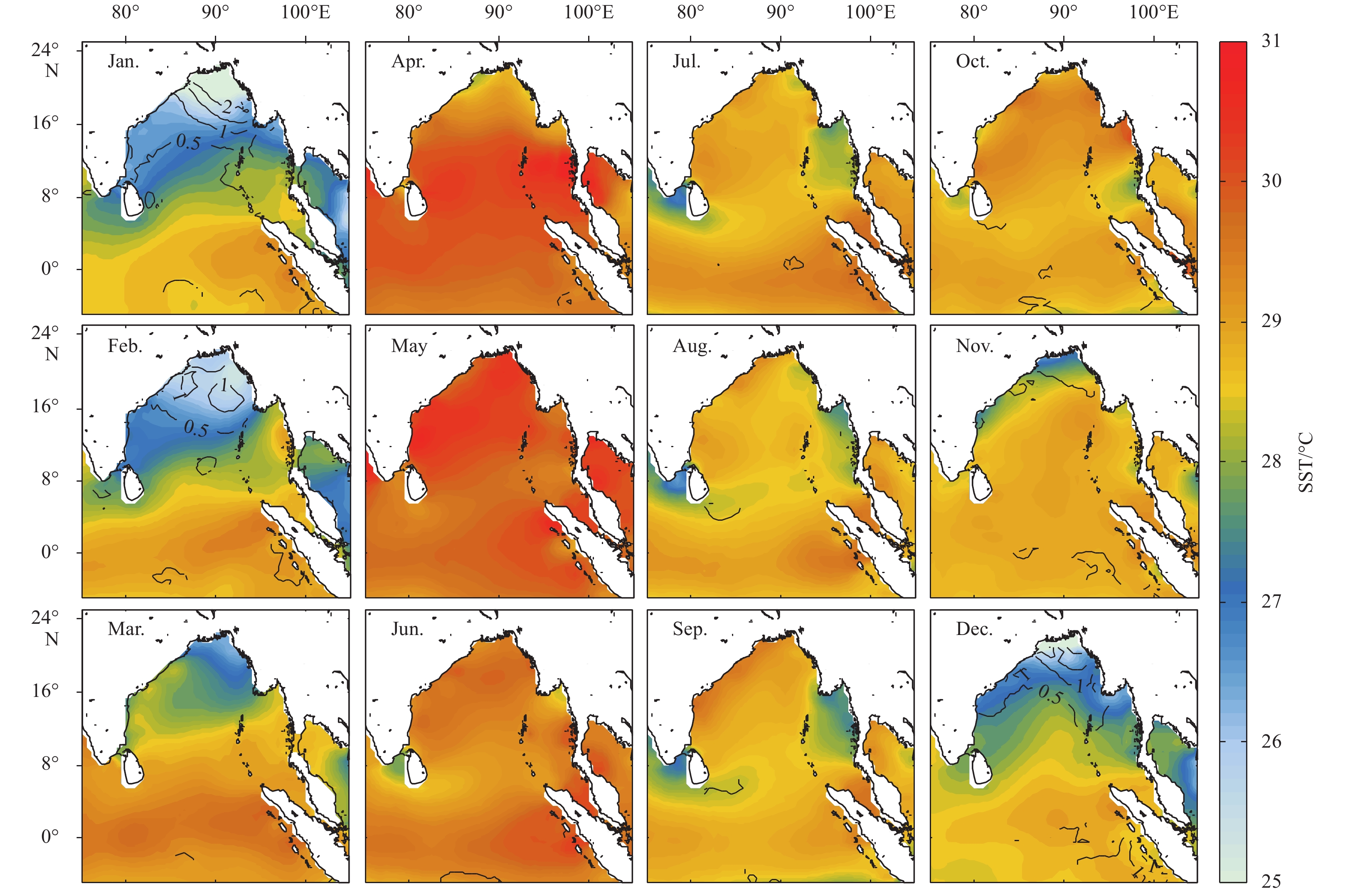
In the BoB, the BL almost disappears from April to May for two reasons. First, affected by the net surface heat flux (NSHF), the SST rises sharply in April and reaches its annual maximum in May (Fig. 3) (Vinayachandran and Shetye, 1991; Liu et al., 2013). The warmer water on the surface with relatively cold water in the subsurface promotes the increase in the vertical temperature gradient, which leads to a shallow IL (of no more than 30 m). Second, at the eastern boundary of the BoB, the coastal upwelling Kelvin waves forced remotely by easterly wind in the EEIO in February drive westward propagating upwelling Rossby waves, causing the IL and ML to rise. From June to September, driven by the southwesterly wind, the surface waters move eastward due to Ekman drift, which causes convergence along the northeastern bay and gradually deepens the IL. Meanwhile, the rainfall in the northeastern BoB reaches the annual maximum value (Varkey et al., 1996), which results in strengthened salinity stratification and a shallow ML. Therefore, a thick BL in excess of 50 m occurs in the northeastern BoB.
Figure
3.
Monthly mean climatology of Argo SST (shading,°C) and temperature inversions (contours,°C). SST: sea surface temperature.
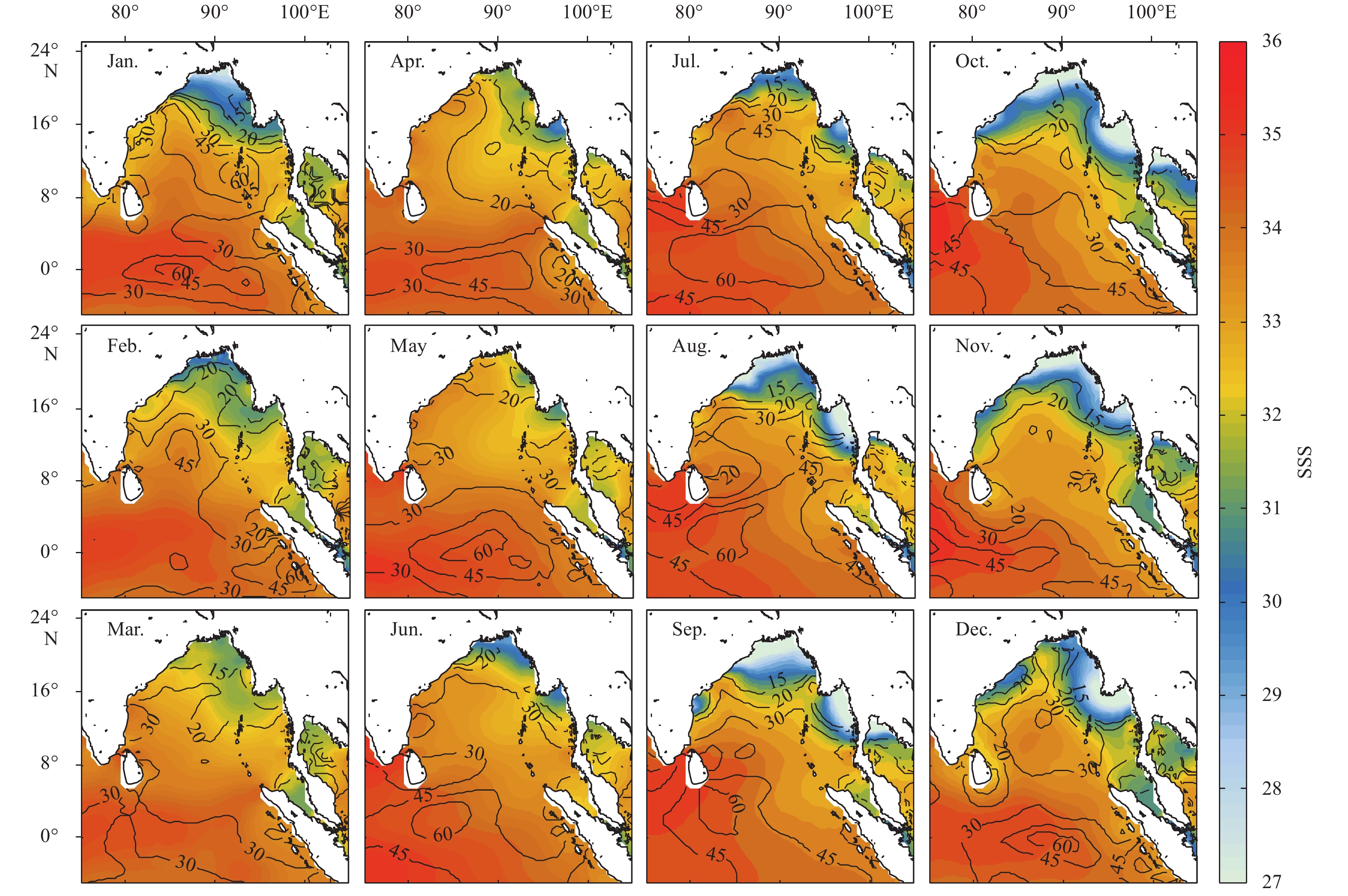
The annual BLT maximum (more than 80 m) in the BoB is observed in January, and the largest spatial extent of the thick BL in excess of 60 m occurs in the northern BoB. Because the ML is very shallow (Fig. 4), the BLT is significantly affected by the ILD. There are three main reasons for the deep IL, which also reaches its annual maximum. First, the coastal downwelling Kelvin waves forced remotely by westerly wind in the EEIO in December radiate westward and propagate downwelling Rossby waves, which deepen the IL. Moreover, the negative wind stress curl reaches its annual maximum in winter, which also deepens the ILD through interior Ekman pumping (Shetye et al., 1993). Finally, affected by the NSHF, the SST reaches its annual minimum (less than 26°C), so the weakened temperature stratification promotes the deepening of the IL. On the other hand, when the SST drops, the vertical distribution of temperature changes to form a subsurface layer of relatively warm water sandwiched between colder waters above and below (Thadathil et al., 2002). Because the downward positive salinity gradient in BL compensates for the stability loss driven by the change in temperature structure, the temperature inversion layer can exist stably in the BL. Influenced by the seasonal cycle of SST, the temperature inversion also reaches its annual maximum (more than 2°C) in January (Fig. 3, contours). In March, as the SST gradually increases, the IL in the BoB becomes shallower, resulting in a relatively thinner BL. In addition, the BL along the boundary of the BoB basically disappears due to the shallower IL caused by coastal upwelling Kelvin waves forced remotely by easterly wind in the EEIO in March. These annual distributions and seasonal cycles of the BLT in the BoB are similar to those described by Thadathil et al. (2007), Agarwal et al. (2012), Kumari et al. (2018), and Shee et al. (2019).
Figure
4.
Monthly mean climatology of Argo SSS (shading, psu) and MLD (contours, m). SSS: sea surface salinity; MLD: mixed layer depth.
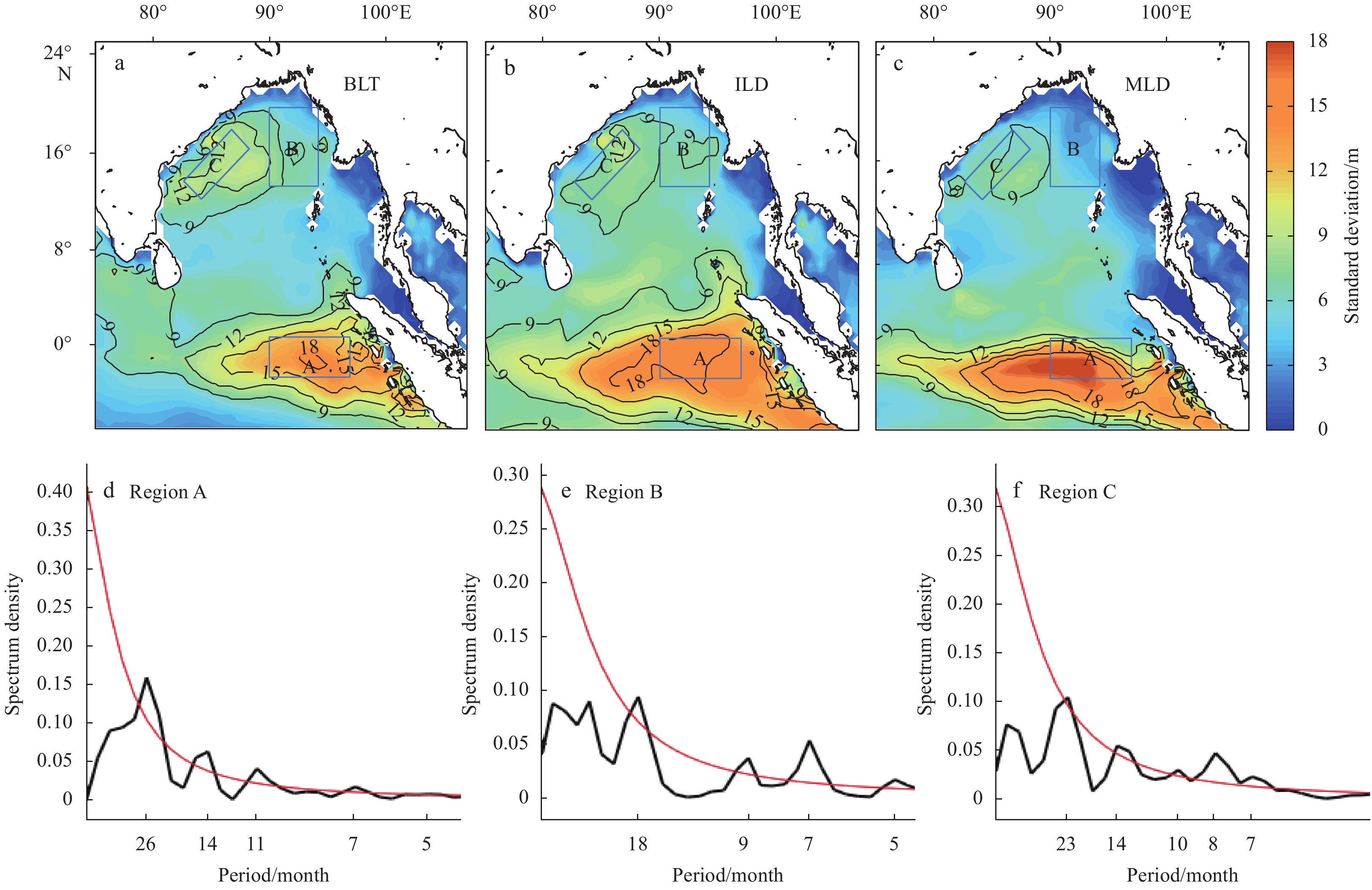
Figures 5a-c (shading) show the standard deviation of the IAV in the BLT, ILD and MLD (subtracted from the climatological annual cycles). There are two large BLT variability regions. The first region is located along the western coast of Sumatra and extends westward (Region A, with an average variance of more than 10 m). Region C is located in the northwestern BoB, and its variance is slightly smaller than that of Region A (more than 8 m). Although the variance in Region B is smaller than that in the other two regions, the thickest BL is found in this region (Fig. 2). Comparison of Figs 5b and c reveal that both the IL and ML contribute to the IAV in the BL in regions A and C, while the IL contributes predominantly in Region C. The contours in Figs 5a-c show the standard deviation of the IAV in the BLT, ILD and MLD during November–February, and the amplitude and distribution are close to those of the total IAV in the BLT, ILD and MLD. This similarity suggests that the variance in the BLT in these months dominates the total interannual variance. Therefore, we only consider November–January (NDJ) variations in Region A and December–February (DJF) variations in Regions B and C. The other reason is that the BLT reaches its annual maximum during these months. Figures 5d-e show the power spectrum for BLT of three regions, and they all have a significant peak for interannual changes (above the 95% confidence level).
Figure
5.
Map of the standard deviation of interannual variability in the BLT, ILD and MLD (a–c). Contours indicate the standard deviation during November–February. Boxes indicate the analysis regions considered in the text. Power spectra for BLT in Regions A–C (d–c). The red lines indicate 95% confidence levels. All variables were removed from the climatological annual cycles. BLT: barrier layer thickness; ILD: isothermal layer depth; MLD: mixed layer depth.
The IOD is an independent ocean-atmosphere coupling mode with strong seasonal phase locking in the Indian Ocean. The IOD usually begins to develop in June, reaches its peak in October and then rapidly disappears (Saji et al., 1999). This phenomenon has good coupling with surface wind and subsurface temperature in the EIO. The surface wind anomaly is related to the Walker circulation anomaly on the basin scale, and the subsurface temperature is usually controlled by marine dynamic processes driven by surface winds, such as Kelvin waves and Rossby waves (Rao et al., 2002). In this study, the dipole mode index (DMI) is calculated using OISST data as the difference between the SST anomalies in the western (10°S–10°N , 50°–70°E) and eastern (10°S–0°N , 90°–110°E) EIO (Saji et al., 1999).
The BLT in the EEIO (Region A in Fig. 5a) has strong interannual variance with a most significant period of 26 months, which falls within the characteristic period of the IOD. Figure 6a shows the time series of BLT, ILD (in NDJ) and DMI (in September-November, SON) anomalies. The BLT and ILD have good correlations with the IOD. The IOD leads the BLT and ILD by two months, and their correlation coefficients reach –0.66 and –0.83, respectively (significant at the 95% level). The positive and negative IOD years are defined based on the DMI normalized by the standard deviation. According to this standard deviation, the positive IOD (pIOD) years were 2006, 2012 and 2015, and the negative IOD (nIOD) years were 2005, 2010 and 2016. Figures 6b and c show the time section of temperature, salinity and ILD, MLD, BLT time series. During pIOD event, although the surface fresh water helps to maintain the strong salinity stratification, which makes the ML very sallow (less than 50 m), the IL also rises, so the BL is abnormally thin. During an nIOD event, both the IL and ML deepen, but affected by local rainfall and current, the ML deepens less due to the salinity stratification that always there all year round, which results in a relatively thick BL (Qiu et al., 2012). Figures 6d and e are similar to Fig. 6b and c) but based on RAMA data. The results are very similar to those of the Argo data.
Figure
6.
a. Time series of BLT, ILD (during NDJ) and DMI (during SON) anomalies. These datasets are standardized and subtracted from the climatological annual cycles. The black dashed lines indicate the standard deviation of the DMI. Time depth section of Argo temperature (b) and salinity (c) averaged in Region A. Time series of ILD (pink line) and MLD (blue line) are shown in (b) and BLT (red line) in (c). Time depth section of RAMA temperature (d) and salinity (e) at 0°, 90°E. Time series of ILD (pink line) and MLD (blue line) are shown in (d) and BLT (red line) in (e). NDJ: Novemberr–January; SON: September–November; BLT: barrier layer thickness; ILD: isothermal layer depth; MLD: mixed layer depth; DMI: dipole mode index.
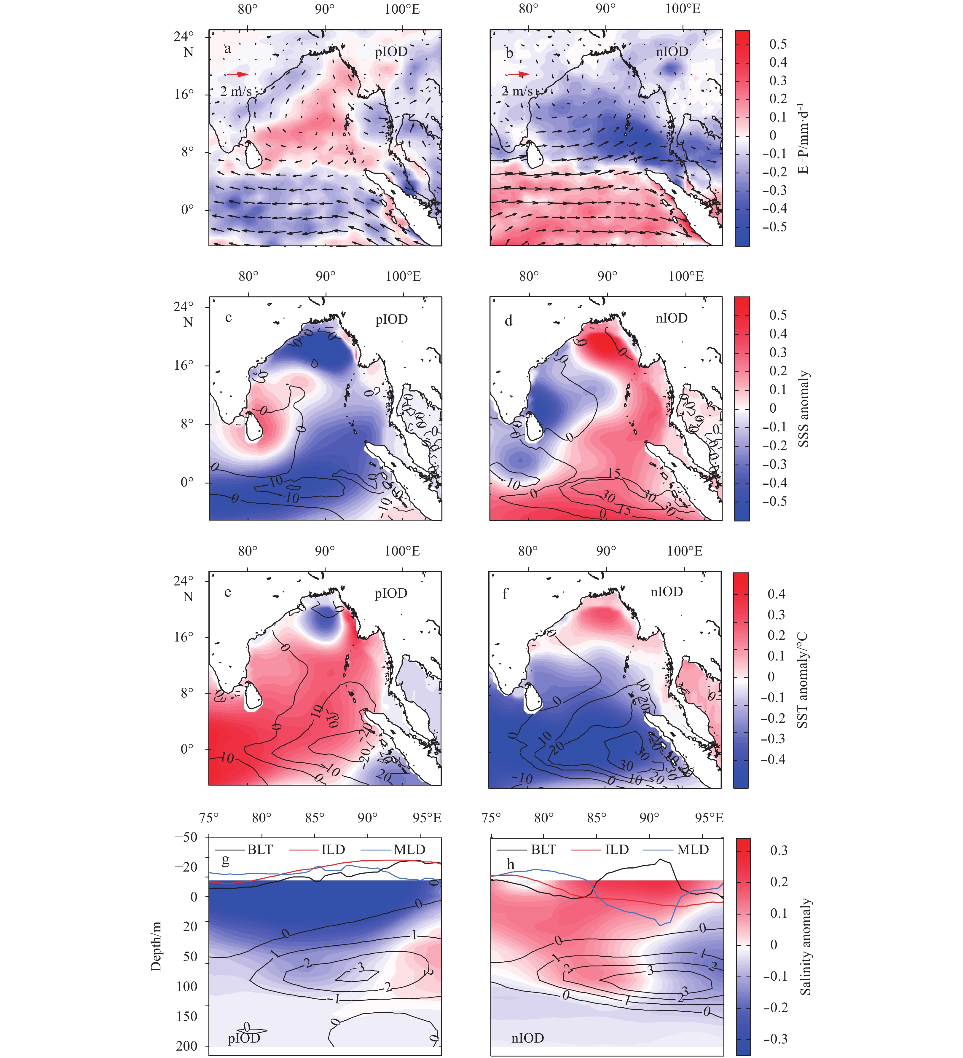
Previous studies suggest that equatorial zonal wind, evaporation minus precipitation (E–P) and the Wyrtki jet have a significant influence on the variations in the BLT in the EEIO (Masson et al., 2002; Qiu et al., 2012; Agarwal et al., 2012). To further examine the dynamic link between IOD and BL in the EEIO, we performed composite analysis of E–P, wind, temperature, salinity, ILD, MLD and BLT anomalies in November-December during pIOD and nIOD events (Fig. 7). During pIOD events, E–P shows negative anomalies in the EEIO, which favors the decrease in SSS (Fig. 7a). At the same time, significant easterly wind anomalies weaken the eastward Wyrtki jet, which reduces the eastward transport of salty water. Therefore, negative salinity anomalies are observed in both the surface and subsurface layers, and the surface salinity decreases more than the subsurface. Due to this increased salinity stratification, the ML shows negative anomalies (more than 10 m) between 80°–93°E (Figs 7c and g). On the other hand, the SST shows a weak positive anomaly (no more than 0.4°C), and the subsurface temperature displays strong positive anomalies (more than 2°C) between 82°–95°E due to eastward-propagating upwelling Kelvin waves associated with easterly wind anomalies. The upwelling Kelvin waves are a forcing factor that lifts the IL, and the negative IL anomalies are slightly larger than the ML anomalies. As a result, a thinner BL is observed (Fig. 7g). These results have also verified the findings of Qiu et al. (2012) who indicate BL is thinner in a pIOD year.
Figure
7.
Composite evaporation minus precipitation (Er–P, shading) and surface wind (vectors) anomalies averaged over ND for pIOD and nIOD (a, b), SSS (shading) and MLD (contours) anomalies (c, d). SST (shading) and ILD (contours) anomalies (e, f), and longitude-depth distribution of salinity (shading) and temperature (contours) anomalies at the equator (g, h). the BLT, ILD and MLD anomalies are superimposed. All variables were removed from the climatological annual cycles. ND: November, December; pIOD: positive IOD year (2006, 2012 and 2015); nIOD: negative IOD year (2005, 2010 and 2016); SSS: sea surface salinity; SST: sea surface temperature; BLT: barrier layer thickness; ILD: isothermal layer depth; MLD: mixed layer depth.
During the nIOD events, similar processes operate but in the opposite direction (Figs 7b, d, f and h). The EEIO shows strong westerly wind anomalies driving downwelling Kelvin waves, resulting in positive subsurface temperature anomalies and abnormal deepening of the IL. Moreover, the SST shows a negative anomaly, which favors the deepening of the IL. Therefore, the ILD shows strong positive anomalies (more than 20 m). However, the variation in ML is relatively complex. The downwelling Kelvin waves and positive SSS anomalies associated with increased E–P are conducive to deepening the ML. On the other hand, westerly wind anomalies strengthen the Wyrtki jet, which carries high-salinity water from the Arabian Sea to the EEIO, and the maximum salinity is in the subsurface layer (Zhang et al., 2015). The positive salinity anomaly in the subsurface layer is slightly greater than that in the surface layer, so the MLD presents a negative anomaly west of 85°E. However, this subsurface positive salinity anomaly has little effect to the east of 85°E. Affected by the flow axis of the Wyrtki jet, the ML shows a strong positive anomaly (more than 30 m) at approximately 2°S, 91°E. The downwelling Kelvin waves and surface positive salinity anomaly contribute to the deepening the ML between 85°E and 93°E, and the positive anomaly of the ML is larger than that of the IL. As a result, the BL shows a negative anomaly between 85°E and 92°E, while it shows a positive anomaly at other longitudes.
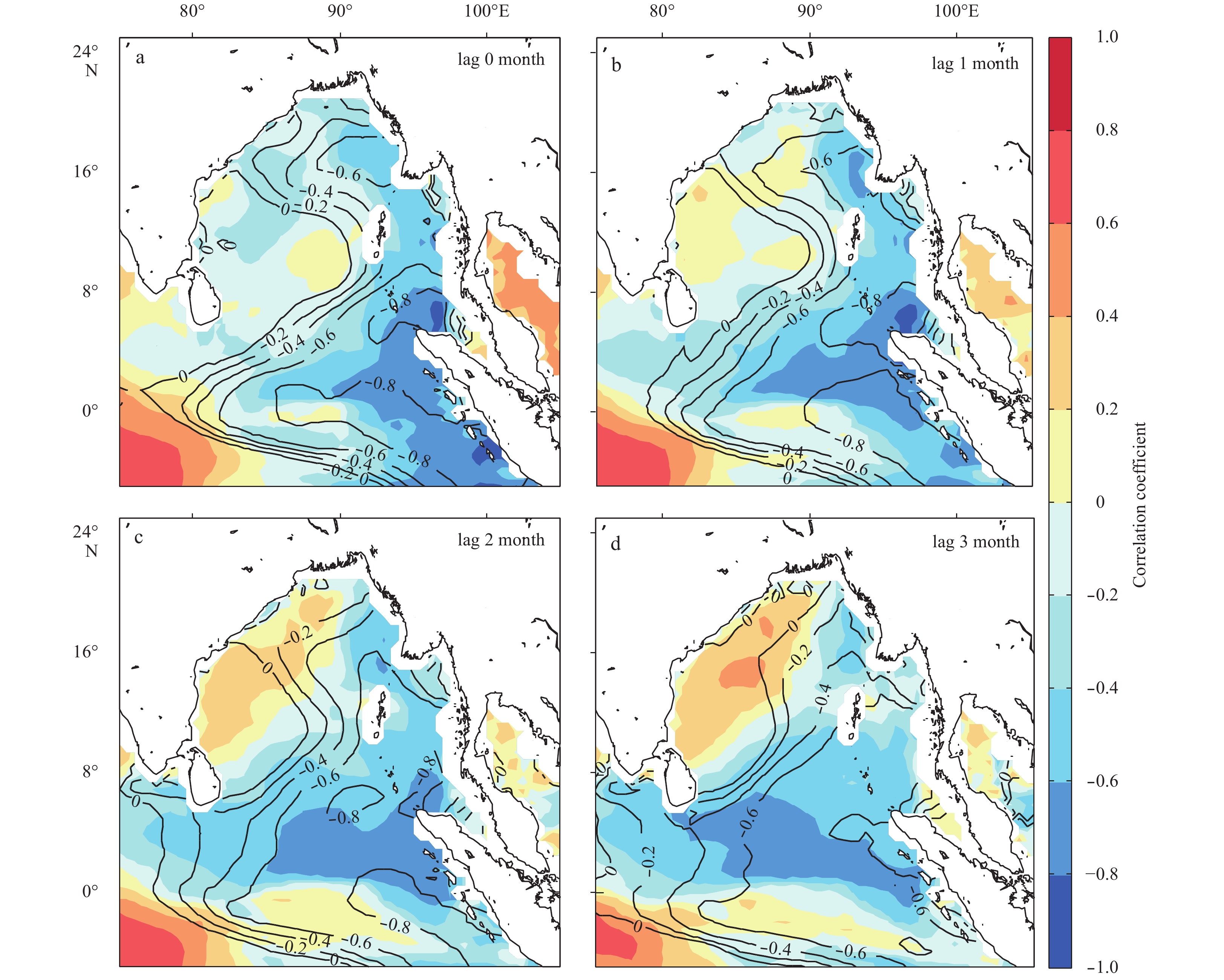
In addition, the ILD has a good relationship with the IOD during both the mature and declining phases of the IOD (Fig. 8), which is similar to the findings of Qiu et al. (2012), who suggested that the IAV in the BLT predominantly results from the IL. However, during nIOD events, we find that the role of the ML should not be ignored and may be more important than that of the IL between 86°E and 92°E along the equator.
Figure
8.
Correlation of the DMI in SON against BLT (shading) and ILD (contours) with 0 (a), 1 (b), 2 (c), and 3 (d) months lag. SON: September–November; BLT: barrier layer thickness; ILD: isothermal layer depth; DMI : dipole mode index.
The analysis in Section 4.1 indicates that there is a close relationship between the BLT in EEIO and IOD on interannual timescales. Previous works have shown that the equatorial westerly (easterly) wind anomalies force the downwelling (upwelling) Kelvin waves to spread to the east, and they turn into coastal Kelvin waves when arriving at Sumatra Island. Then, the waves propagate northward to the eastern and northern boundaries of the BoB. In addition, at the northern end of Burma’s Irrawaddy delta, the coastal Kelvin waves radiate Rossby waves that cause positive (negative) anomalies in the ILD in the BoB. The waves take about a month to propagate from EEIO to the northeast of BoB (Cheng et al., 2013, 2017; Rao et al., 2010; Suresh et al., 2016). Consequently, during the strong pIOD (nIOD) years, a thin (thick) BL appears in the BoB and lags behind the variation in zonal wind stress by approximately one month (Rao et al., 2010; Cai et al., 2013; Cyriac et al., 2016; Kumari et al., 2018). Indeed, when the BLT in the eastern and northeastern BoB is modeled as lagging behind the IOD by one month, they exhibit a good coupling relationship (Fig. 8b). However, their correlation is significantly weaker with a three-month lag (Fig. 8d). This is because the IOD has decayed in December, so it may not have a significant impact on the IAV in BLT in winter.
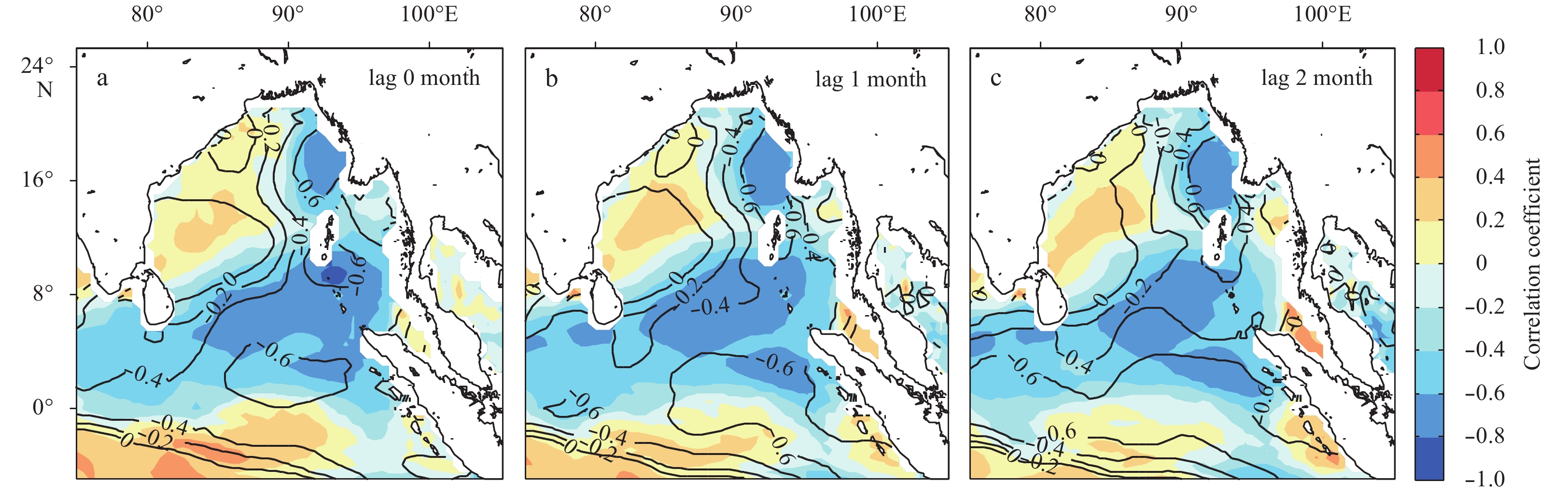
Previous studies have shown that warm (cold) SST anomalies in the tropical eastern Pacific cause easterly (westerly) wind anomalies in the EEIO via convection-driven Walker circulation (Wang et al., 2000; Xie et al., 2002, 2016). Yuan and Su (2019) indicate that ENSO could influence the varibility in BLT by affecting the thermocline, especially in the eastern tropical Indian Ocean. Considering that the mature phase of ENSO is in winter (NDJ) (Wang et al., 2000), the IAV in DJF BLT may be associated with ENSO. The IAV in the BLT and ILD (in DJF) in the northeastern BoB shows a good correspondence with the Niño 3.4 index (Fig. 9). In Region B, the variance in MLD is very small (less than 4 m, Fig. 5), so we only need to pay attention to the ILD. Figure 10a shows the correlation between ILD and the averaged zonal wind stress within the blue box (1°S–1°N, 80°–90°E). There is a relatively good correspondence between the ILD (in DJF) and the equatorial zonal wind stress (in NDJ), and their correlation coefficients reach 0.6 (significant at the 95% confidence level, Fig. 10c). Equatorial zonal wind stress anomalies associated with ENSO can explain the variance in ILD in Region B to a great extent.
Figure
9.
Correlation of the Niño 3.4 index in NDJ and BLT (shading) or ILD (contours) with 0 (a), 1 (b), and 2 (c) months lag. NDJ: November–January; BLT: barrier layer thickness; ILD: isothermal layer depth.
Figure
10.
Correlation of the zonal wind stress (in NDJ) averaged in the blue box (1°S–1°N, 80°–90°E) against ILD (in DJF) in each grid (a); correlation of the zonal wind stress (in DJF) against ILD (in DJF) (b); and time series of ILD (in DJF, black line, within the black box), zonal wind stress (in DJF, blue line, within the blue box) and Niño 3.4 index (in NDJ, red line) anomalies (c). All variables were standardized, and the climatological annual cycles were removed. NDJ: November–January; DJF: December–February; ILD: isothermal layer depth.
The BLT in the northwestern BoB (Region C) shows strong interannual variance. In this area, the ILD variations are likely related to wind stress curl in the northern BoB. Figures 11a-c display the correlations of BLT, ILD and MLD with the averaged wind stress curl in the blue box, lagging the wind stress curl by one month. The positive (negative) ILD anomalies clearly correspond well to negative (positive) wind stress curl. The correlation coefficient between the wind stress curl in the blue box and the BLT in the black box is –0.7 (Fig. 11g), and the correlation coefficient between the wind stress curl and the Niño 3.4 index is –0.44 (significant at the 95% level, Fig. 11h). The BLT in the black box also has a significant correlation with the wind speed in the blue box (r=0.48, Fig. 11g).
Figure
11.
Correlations between the wind stress curl (in DJF) within the blue box (11°–21°N, 83°–95°E) and BLT (a), ILD (b) and MLD (c) (in JFM), respectively, in each grid; correlations between the wind speed (in DJF) within the blue box and BLT (d), ILD (e) and MLD (f) (in JFM), respectively, in each grid; time series of wind stress curl (in DJF, black line, within the blue box), wind speed (in DJF, blue line, within the blue box) and BLT (in JFM, red line, within the black box) anomalies (g); and time series of wind stress curl (in DJF, black line, within the blue box) and Niño 3.4 index (in NDJ, red line) anomalies (h). All variables were standardized, and the climatological annual cycles were removed. DJF: December–February; JFM: January-March; BLT: barrier layer thickness; ILD: isothermal layer depth; MLD: mixed layer depth.
The stronger (weaker) northeasterly wind transports more (less) surface fresh water from the northeast of the BoB to the west, strengthening (weakening) the salinity stratification in Region C, which causes the ML to abnormally shallow (deepen). However, the strong (weak) wind stress means strong (weak) convective mixing, which causes the ML to abnormally deepen (shallow). Because these two effects might offset each other, there is a very weak correlation between wind speed and MLD in Region C (Fig. 11f). In contrast, stronger (weaker) northeasterly winds increase (decrease) the westward Ekman transport, which leads to deeper (shallower) IL and ML through the process of convergence (divergence). Easterly (westerly) wind anomalies in the EEIO associated with a positive (negative) ENSO phase strengthens (weakens) the anticyclone in the BoB. Furthermore, the negative (positive) wind stress curl through the interior (exterior) Ekman pumping further increases (decreases) the ILD and MLD. The ILD (BLT) in the western BoB is also affected by the superposition effect of westward Rossby waves radiated by coastal Kelvin waves along the eastern coast. In general, the local wind field in winter is the key factor in modulating the BLT in the western BoB on interannual timescales. Considering the adjustment of the ocean to atmospheric forcing, the response is delayed by a month. Figure 11 indicates that the surface wind forcing in the northern BoB dominates the IAV in the winter ILD in Region C. Because the ML variability is very weak, the IAV in the BLT is mainly determined by the ILD.
5.
Summary and conclusions
Argo grid data from 2002–2017 are used to investigate the seasonal variability and IAV in the BLT in the EEIO and BoB and the associated forcing mechanisms. The observed evolution of the BLT displays obvious seasonal changes, with maxima during NDJ in the EEIO and during DJF in the north of BoB, in agreement with the conclusions of previous studies. Therefore, we focus on its variation in winter.
Strong IAV in the BLT with a large amplitude was observed in EEIO, and this variability is associated with the IOD. During the pIOD phase, the thin BL is mainly affected by the ILD, which is modulated by upwelling Kelvin waves associated with the easterly wind anomaly, which is similar to Qiu et al. (2012). During the nIOD phase, the downwelling Kelvin waves driven by westerly anomaly deepen the IL. However, the variability of MLD is somewhat complex. The ML west of 85°E has negative anomaly due to high subsurface salinity water taken by the Wyrtki jet from west. Therefore, the BLT shows a negative anomaly between 86°E and 92°E but shows a positive anomaly at other longitudes.
The equatorial zonal wind stress anomaly regulated by ENSO remotely affects the IAV in the BLT in the eastern and northeastern BoB by driving Kelvin waves and Rossby waves. In the western BoB, the local wind field is also modulated by ENSO, which is the key factor controlling the BLT.
Agarwal N, Sharma R, Parekh A, et al. 2012. Argo observations of barrier layer in the tropical Indian Ocean. Advances in Space Research, 50(5): 642–654. doi: 10.1016/j.asr.2012.05.021
[2]
Breugem W P, Chang P, Jang C J, et al. 2008. Barrier layers and tropical Atlantic SST biases in coupled GCMs. Tellus A, 60(5): 885–897. doi: 10.1111/j.1600-0870.2008.00343.x
[3]
Cai W, Pan A, Roemmich D, et al. 2009. Argo profiles a rare occurrence of three consecutive positive Indian Ocean Dipole events, 2006–2008. Geophysical Research Letters, 36(8): L08701. doi: 10.1029/2008GL037038
[4]
Cai Wenju, Zheng Xiaotong, Weller E, et al. 2013. Projected response of the Indian Ocean Dipole to greenhouse warming. Nature Geoscience, 6(12): 999–1007. doi: 10.1038/ngeo2009
[5]
Cheng Xuhua, McCreary J P, Qiu Bo, et al. 2017. Intraseasonal-to-semiannual variability of sea-surface height in the astern, equatorial Indian Ocean and southern Bay of Bengal. Journal of Geophysical Research, 122(5): 4051–4067. doi: 10.1002/2016JC012662
[6]
Cheng Xuhua, Xie Shangping, McCreary J P, et al. 2013. Intraseasonal variability of sea surface height in the Bay of Bengal. Journal of Geophysical Research, 118(2): 816–830. doi: 10.1002/jgrc.20075
[7]
Chowdary J S, Gnanaseelan C, Xie S P. 2009. Westward propagation of barrier layer formation in the 2006-07 Rossby wave event over the tropical southwest Indian Ocean. Geophysical Research Letters, 36(4): L04607. doi: 10.1029/2008GL036642
[8]
Cyriac A, Ghoshal T, Shaileshbhai P R, et al. 2016. Variability of sensible heat flux over the Bay of Bengal and its connection to Indian Ocean Dipole events. Ocean Science Journal, 51(1): 97–107. doi: 10.1007/s12601-016-0009-9
[9]
De Boyer Montegut C, Mignot J, Lazar A, et al. 2007. Control of salinity on the mixed layer depth in the world ocean: 1. General description. Journal of Geophysical Research, 112(C6): C06011. doi: 10.1029/2006JC003953
[10]
Dee D P, Uppala S M, Simmons A J, et al. 2011. The ERA-Interim reanalysis: configuration and performance of the data assimilation system. Quarterly Journal of the Royal Meteorological Society, 137(656): 553–597. doi: 10.1002/qj.828
[11]
Fousiya T S, Parekh A, Gnanaseelan C. 2016. Interannual variability of upper ocean stratification in Bay of Bengal: observational and modeling aspects. Theoretical and Applied Climatology, 126: 285–301. doi: 10.1007/s00704-015-1574-z
[12]
Gaillard F, Reynaud T, Thierry V, et al. 2016. In situ-based reanalysis of the global ocean temperature and salinity with ISAS: variability of the heat content and steric height. Journal of Climate, 29(4): 1305–1323. doi: 10.1175/JCLI-D-15-0028.1
[13]
Girishkumar M S, Ravichandran M, McPhaden M J, et al. 2011. Intraseasonal variability in barrier layer thickness in the south central Bay of Bengal. Journal of Geophysical Research, 116(3): C03009. doi: 10.1029/2010JC006657
[14]
Girishkumar M S, Ravichandran M, McPhaden M J. 2013. Temperature inversions and their influence on the mixed layer heat budget during the winters of 2006–2007 and 2007–2008 in the Bay of Bengal. Journal of Geophysical Research, 118(5): 2426–2437. doi: 10.1002/jgrc.20192
[15]
Godfrey J S, Lindstrom E J. 1989. The heat budget of the equatorial western Pacific surface mixed layer. Journal of Geophysical Research, 94(C6): 8007–8017. doi: 10.1029/JC094iC06p08007
[16]
Jiang Xingwen, Li Jianping. 2011. Influence of the annual cycle of sea surface temperature on the monsoon onset. Journal of Geophysical Research, 116(D10): D10105. doi: 10.1029/2010JD015236
[17]
Kara A B, Rochford P A, Hurlburt H E. 2000. An optimal definition for ocean mixed layer depth. Journal of Geophysical Research, 105(C7): 16803–16821. doi: 10.1029/2000JC900072
[18]
Kumari A, Prasanna Kumar S, Chakraborty A. 2018. Seasonal and interannual variability in the barrier layer of the bay of Bengal. Journal of Geophysical Research, 123(2): 1001–1015. doi: 10.1002/2017JC013213
[19]
Li T, Zhang Yongsheng, Chang C P, et al. 2001. On the relationship between Indian ocean sea surface temperature and Asian summer monsoon. Geophysical Research Letters, 28(14): 2843–2846. doi: 10.1029/2000GL011847
[20]
Lindstrom E, Lukas R, Fine R, et al. 1987. The western equatorial Pacific Ocean circulation study. Nature, 300(6148): 533–537
[21]
Liu Yanliang, Yu Weidong, Li Kuiping, et al. 2013. Mixed layer heat budget in Bay of Bengal: Mechanism of the generation and decay of spring warm pool. Haiyang Xuebao (in Chinese), 35(6): 1–8
[22]
Lukas R, Lindstrom E. 1991. The mixed layer of the western equatorial Pacific Ocean. Journal of Geophysical Research, 96(S01): 3343–3357. doi: 10.1029/90JC01951
[23]
Maes C, Picaut J, Belamari S. 2005. Importance of the salinity barrier layer for the buildup of EL Niño. Journal of Climate, 18(1): 104–118. doi: 10.1175/JCLI-3214.1
[24]
Masson S, Delecluse P, Boulanger J P, et al. 2002. A model study of the seasonal variability and formation mechanisms of the barrier layer in the eastern equatorial Indian Ocean. Journal of Geophysical Research, 107(C12): 8017. doi: 10.1029/2001JC000832
[25]
McPhaden M J, Meyers G, Ando K, el al. 2009. RAMA: the research moored array for African-Asian-Australian monsoon analysis and prediction. Bulletin of the American Meteorological Society, 90(4): 459–480. doi: 10.1175/2008BAMS2608.1
[26]
Oppo D W, Rosenthal Y, Linsley B K. 2009. 2,000-year-long temperature and hydrology reconstructions from the Indo-Pacific warm pool. Nature, 460(7259): 1113–1116. doi: 10.1038/nature08233
[27]
Palmer T N, Mansfield D A. 1984. Response of two atmospheric general circulation models to sea-surface temperature anomalies in the tropical east and west Pacific. Nature, 310(5977): 483–485. doi: 10.1038/310483a0
[28]
Pang Shanshan, Wang Xidong, Liu Hailong, et al. 2019. Decadal variability of the barrier layer and forcing mechanism in the Bay of Bengal. Journal of Geophysical Research, 124(7): 5289–5307. doi: 10.1029/2018JC014918
[29]
Qiu Yun, Cai Wenju, Li Li, et al. 2012. Argo profiles variability of barrier layer in the tropical Indian Ocean and its relationship with the Indian Ocean Dipole. Geophysical Research Letters, 39(8): L08605. doi: 10.1029/2012GL051441
[30]
Qu Tangdong, Meyers G. 2005. Seasonal variation of barrier layer in the southeastern tropical Indian Ocean. Journal of Geophysical Research, 110(C11): C11003. doi: 10.1029/2004JC002816
[31]
Rao S A, Behera S K, Masumoto Y, et al. 2002. Interannual subsurface variability in the tropical Indian Ocean with a special emphasis on the Indian Ocean Dipole. Deep Sea Research Part II: Topical Studies in Oceanography, 49(7–8): 1549–1572. doi: 10.1016/S0967-0645(01)00158-8
[32]
Rao R R, Girish Kumar M S, Ravichandran M, et al. 2010. Interannual variability of Kelvin wave propagation in the wave guides of the equatorial Indian Ocean, the coastal Bay of Bengal and the southeastern Arabian Sea during 1993-2006. Deep Sea Research Part I: Oceanographic Research Papers, 57(1): 1–13. doi: 10.1016/j.dsr.2009.10.008
[33]
Rao R R, Sivakumar R. 2003. Seasonal variability of sea surface salinity and salt budget of the mixed layer of the north Indian Ocean. Journal of Geophysical Research, 108(C1): 3009. doi: 10.1029/2001JC000907
[34]
Saji N H, Goswami B N, Vinayachandran P N, et al. 1999. A dipole mode in the tropical Indian Ocean. Nature, 401(6751): 360–363
[35]
Shankar D, Shetye S R, Joseph P V. 2007. Link between convection and meridional gradient of sea surface temperature in the Bay of Bengal. Journal of Earth System Science, 116(5): 385–406. doi: 10.1007/s12040-007-0038-y
[36]
Shee A, Sil S, Gangopadhyay A, et al. 2019. Seasonal evolution of oceanic upper layer processes in the northern Bay of Bengal following a single Argo float. Geophysical Research Letters, 46(10): 5369–5377. doi: 10.1029/2019GL082078
[37]
Shenoi S S C, Shankar D, Shetye S R. 2002. Differences in heat budgets of the near-surface Arabian Sea and Bay of Bengal: Implications for the summer monsoon. Journal of Geophysical Research, 107(C6): 3052. doi: 10.1029/2000JC000679
[38]
Shetye S R, Gouveia A D, Shenoi S S C, et al. 1993. The western boundary current of the seasonal subtropical gyre in the Bay of Bengal. Journal of Geophysical Research, 98(C1): 945–954. doi: 10.1029/92JC02070
[39]
Sprintall J, Tomczak M. 1992. Evidence of the barrier layer in the surface layer of the tropics. Journal of Geophysical Research, 97: 7305–7316. doi: 10.1029/92JC00407
[40]
Suresh I, Vialard J, Izumo T, et al. 2016. Dominant role of winds near Sri Lanka in driving seasonal sea level variations along the west coast of India. Geophysical Research Letters, 43(13): 7028–7035. doi: 10.1002/2016GL069976
[41]
Thadathil P, Gopalakrishna V V, Muraleedharan P M, et al. 2002. Surface layer temperature inversion in the Bay of Bengal. Deep Sea Research Part I: Oceanographic Research Papers, 49(10): 1801–1818. doi: 10.1016/S0967-0637(02)00044-4
[42]
Thadathil P, Muraleedharan P M, Rao R R, et al. 2007. Observed seasonal variability of barrier layer in the Bay of Bengal. Journal of Geophysical Research, 112(C2): C02009. doi: 10.1029/2006JC003651
[43]
Thangaprakash V P, Girishkumar M S, Suprit K, et al. 2016. What controls seasonal evolution of sea surface temperature in the Bay of Bengal? Mixed layer heat budget analysis using moored buoy observations along 90°E Oceanography, 29(2): 202–213. doi: 10.5670/oceanog.2016.52
[44]
Thompson B, Gnanaseelan C, Salvekar P S. 2006. Seasonal evolution of temperature inversions in the north Indian Ocean. Current Science, 90(5): 697–704
[45]
Valsala V, Singh S, Balasubramanian S. 2018. A modeling study of interannual variability of Bay of Bengal mixing and barrier layer formation. Journal of Geophysical Research, 123(6): 3962–3981. doi: 10.1029/2017JC013637
[46]
Varkey M J, Murty V S N, Suryanarayana A. 1996. Physical oceanography of the Bay of Bengal and Andaman sea. Oceanography and Marine Biology: An Annual Review, 34: 1–70
[47]
Vialard J, Delecluse P. 1998. An OGCM study for the TOGA decade. Part I: role of salinity in the physics of the Western Pacific fresh pool. Journal of Physical Oceanography, 28(6): 1071–1088
[48]
Vinayachandran P N, Murty V S N, Ramesh Babu V. 2002. Observations of barrier layer formation in the Bay of Bengal during summer monsoon. Journal of Geophysical Research, 107(C12): 8018. doi: 10.1029/2001JC000831
[49]
Vinayachandran P N, Shetye S R. 1991. The warm pool in the Indian Ocean. Proceedings of the Indian Academy of Sciences—Earth and Planetary Sciences, 100(2): 165–175
[50]
Wang Bin, Wu Renguang, Fu Xiouhua. 2000. Pacific-East Asian teleconnection: how does ENSO affect East Asian climate? Journal of Climate, 13(9): 1517–1536. doi: 10.1175/1520-0442(2000)013<1517:PEATHD>2.0.CO;2
[51]
Wyrtki K. 1973. An equatorial jet in the Indian Ocean. Science, 181(4096): 262–264. doi: 10.1126/science.181.4096.262
[52]
Xie Shangping, Annamalai H, Schott F A, et al. 2002. Structure and mechanisms of south Indian Ocean climate variability. Journal of Climate, 15(8): 864–878. doi: 10.1175/1520-0442(2002)015<0864:SAMOSI>2.0.CO;2
[53]
Xie Shangping, Kosaka Y, Du Yan, et al. 2016. Indo-western Pacific ocean capacitor and coherent climate anomalies in post-ENSO summer: a review. Advances in Atmospheric Sciences, 33(4): 411–432. doi: 10.1007/s00376-015-5192-6
You Yuzhu. 1995. Salinity variability and its role in the barrier-layer formation during TOGA-COARE. Journal of Physical Oceanography, 25(11): 2778–2807. doi: 10.1175/1520-0485(1995)025<2778:SVAIRI>2.0.CO;2
[56]
You Yuzhu. 1998. Rain-formed barrier layer of the western equatorial Pacific Warm Pool: a case study. Journal of Geophysical Research, 103(C3): 5361–5378. doi: 10.1029/97JC03421
[57]
Yuan Xu, Su Zhongbo. 2019. The seasonal and interannual variabilities of the barrier layer thickness in the tropical Indian Ocean. Ocean Science, : doi: 10.5194/os-2019-12
[58]
Zhang Ying, Du Yan, Zhang Yuhong, et al. 2015. Asymmetric influences of positive and negative IOD events on salinity transport by the fall Wyrtki Jet along the equatorial Indian Ocean. Journal of Tropical Oceanography (in Chinese), 34(5): 1–10
Zhiyuan Li, Yu Long, Saihua Huang, et al. A Large Winter Chlorophyll‐a Bloom in the Southeastern Bay of Bengal Associated With the Extreme Indian Ocean Dipole Event in 2019. Journal of Geophysical Research: Oceans, 2023, 128(3) doi:10.1029/2022JC018791
2.
Jifeng Qi, Tangdong Qu, Baoshu Yin. Meta-learning-based estimation of the barrier layer thickness in the tropical Indian Ocean. Environmental Research Communications, 2023, 5(9): 091005. doi:10.1088/2515-7620/acf9e1
3.
Biplab Sadhukhan, Arun Chakraborty. Role of local and remote forcing on the decadal variability of Mixed Layer Depth in the Bay of Bengal. Dynamics of Atmospheres and Oceans, 2023, 102: 101349. doi:10.1016/j.dynatmoce.2022.101349
4.
Priyambada Chutia, Manas Das, Nabajyoti Goswami, et al. Deciphering the role of aquaporin 1 in the adaptation of the stinging catfish Heteropneustes fossilis to environmental hypertonicity by molecular dynamics simulation studies. Journal of Biomolecular Structure and Dynamics, 2023, 41(6): 2075. doi:10.1080/07391102.2022.2027272
5.
Vinu Valsala, A. G. Prajeesh, Shikha Singh. Numerical Investigation of Tropical Indian Ocean Barrier Layer Variability. Journal of Geophysical Research: Oceans, 2022, 127(10) doi:10.1029/2022JC018637
6.
Lanman Li, Xuhua Cheng, Zhiyou Jing, et al. Submesoscale motions and their seasonality in the northern Bay of Bengal. Acta Oceanologica Sinica, 2022, 41(4): 1. doi:10.1007/s13131-021-1847-6
Tian Ma, Xuhua Cheng, Yiquan Qi, Jiajia Chen. Interannual variability in the barrier layer and forcing mechanism in the eastern equatorial Indian Ocean and Bay of Bengal[J]. Acta Oceanologica Sinica, 2020, 39(7): 19-31. doi: 10.1007/s13131-020-1575-3
Tian Ma, Xuhua Cheng, Yiquan Qi, Jiajia Chen. Interannual variability in the barrier layer and forcing mechanism in the eastern equatorial Indian Ocean and Bay of Bengal[J]. Acta Oceanologica Sinica, 2020, 39(7): 19-31. doi: 10.1007/s13131-020-1575-3
Figure 1. Correlation coefficients for BLT, ILD and MLD between Argo grid data and RAMA data at 0°, 90°E and 15°N, 90°E. BLT: barrier layer thickness; ILD: isothermal layer depth; MLD: mixed layer depth.
Figure 2. Monthly mean climatology of Argo BLT (shading, m), ILD (contours, m) and ECMWF surface winds (vectors, m/s). BLT: barrier layer thickness; ILD: isothermal layer depth.
Figure 3. Monthly mean climatology of Argo SST (shading,°C) and temperature inversions (contours,°C). SST: sea surface temperature.
Figure 4. Monthly mean climatology of Argo SSS (shading, psu) and MLD (contours, m). SSS: sea surface salinity; MLD: mixed layer depth.
Figure 5. Map of the standard deviation of interannual variability in the BLT, ILD and MLD (a–c). Contours indicate the standard deviation during November–February. Boxes indicate the analysis regions considered in the text. Power spectra for BLT in Regions A–C (d–c). The red lines indicate 95% confidence levels. All variables were removed from the climatological annual cycles. BLT: barrier layer thickness; ILD: isothermal layer depth; MLD: mixed layer depth.
Figure 6. a. Time series of BLT, ILD (during NDJ) and DMI (during SON) anomalies. These datasets are standardized and subtracted from the climatological annual cycles. The black dashed lines indicate the standard deviation of the DMI. Time depth section of Argo temperature (b) and salinity (c) averaged in Region A. Time series of ILD (pink line) and MLD (blue line) are shown in (b) and BLT (red line) in (c). Time depth section of RAMA temperature (d) and salinity (e) at 0°, 90°E. Time series of ILD (pink line) and MLD (blue line) are shown in (d) and BLT (red line) in (e). NDJ: Novemberr–January; SON: September–November; BLT: barrier layer thickness; ILD: isothermal layer depth; MLD: mixed layer depth; DMI: dipole mode index.
Figure 7. Composite evaporation minus precipitation (Er–P, shading) and surface wind (vectors) anomalies averaged over ND for pIOD and nIOD (a, b), SSS (shading) and MLD (contours) anomalies (c, d). SST (shading) and ILD (contours) anomalies (e, f), and longitude-depth distribution of salinity (shading) and temperature (contours) anomalies at the equator (g, h). the BLT, ILD and MLD anomalies are superimposed. All variables were removed from the climatological annual cycles. ND: November, December; pIOD: positive IOD year (2006, 2012 and 2015); nIOD: negative IOD year (2005, 2010 and 2016); SSS: sea surface salinity; SST: sea surface temperature; BLT: barrier layer thickness; ILD: isothermal layer depth; MLD: mixed layer depth.
Figure 8. Correlation of the DMI in SON against BLT (shading) and ILD (contours) with 0 (a), 1 (b), 2 (c), and 3 (d) months lag. SON: September–November; BLT: barrier layer thickness; ILD: isothermal layer depth; DMI : dipole mode index.
Figure 9. Correlation of the Niño 3.4 index in NDJ and BLT (shading) or ILD (contours) with 0 (a), 1 (b), and 2 (c) months lag. NDJ: November–January; BLT: barrier layer thickness; ILD: isothermal layer depth.
Figure 10. Correlation of the zonal wind stress (in NDJ) averaged in the blue box (1°S–1°N, 80°–90°E) against ILD (in DJF) in each grid (a); correlation of the zonal wind stress (in DJF) against ILD (in DJF) (b); and time series of ILD (in DJF, black line, within the black box), zonal wind stress (in DJF, blue line, within the blue box) and Niño 3.4 index (in NDJ, red line) anomalies (c). All variables were standardized, and the climatological annual cycles were removed. NDJ: November–January; DJF: December–February; ILD: isothermal layer depth.
Figure 11. Correlations between the wind stress curl (in DJF) within the blue box (11°–21°N, 83°–95°E) and BLT (a), ILD (b) and MLD (c) (in JFM), respectively, in each grid; correlations between the wind speed (in DJF) within the blue box and BLT (d), ILD (e) and MLD (f) (in JFM), respectively, in each grid; time series of wind stress curl (in DJF, black line, within the blue box), wind speed (in DJF, blue line, within the blue box) and BLT (in JFM, red line, within the black box) anomalies (g); and time series of wind stress curl (in DJF, black line, within the blue box) and Niño 3.4 index (in NDJ, red line) anomalies (h). All variables were standardized, and the climatological annual cycles were removed. DJF: December–February; JFM: January-March; BLT: barrier layer thickness; ILD: isothermal layer depth; MLD: mixed layer depth.


 DownLoad: