

-
Abstract: With the development of satellite altimetry technology, the resolution of sea-level anomaly (SLA) datasets is constantly improving. Current spatial resolution levels can reach a grid size of (1/4)° × (1/4)°, with daily measurements that span from 1993 to 2018, allowing for the precise identification and tracking of individual eddies. In the current study, in addition to the internal circulation and migration of eddies, a new aspect in eddy kinematics is revealed and investigated for the first time: shape-based overall eddy rotation (SOER), based on the intrinsic elliptical shape of eddies identified from a high-resolution SLA dataset. We found that eddies can maintain an elliptical shape and a slow and stable SOER during their migration process. The SOER speed was observed to be negatively correlated to eddy lifetime, and exhibited a dependence on latitude, decreasing from low- and high- to mid-latitudes. The SOER direction tended to be consistent with the direction of internal circulation, particularly for long-lived eddies. In addition, we identified a negative relationship between internal circulation speed and SOER speed while the migration speed was positively related to SOER speed. These findings further expand and improve eddy kinematics, which is of great significance for the future study of eddy dynamics.
-
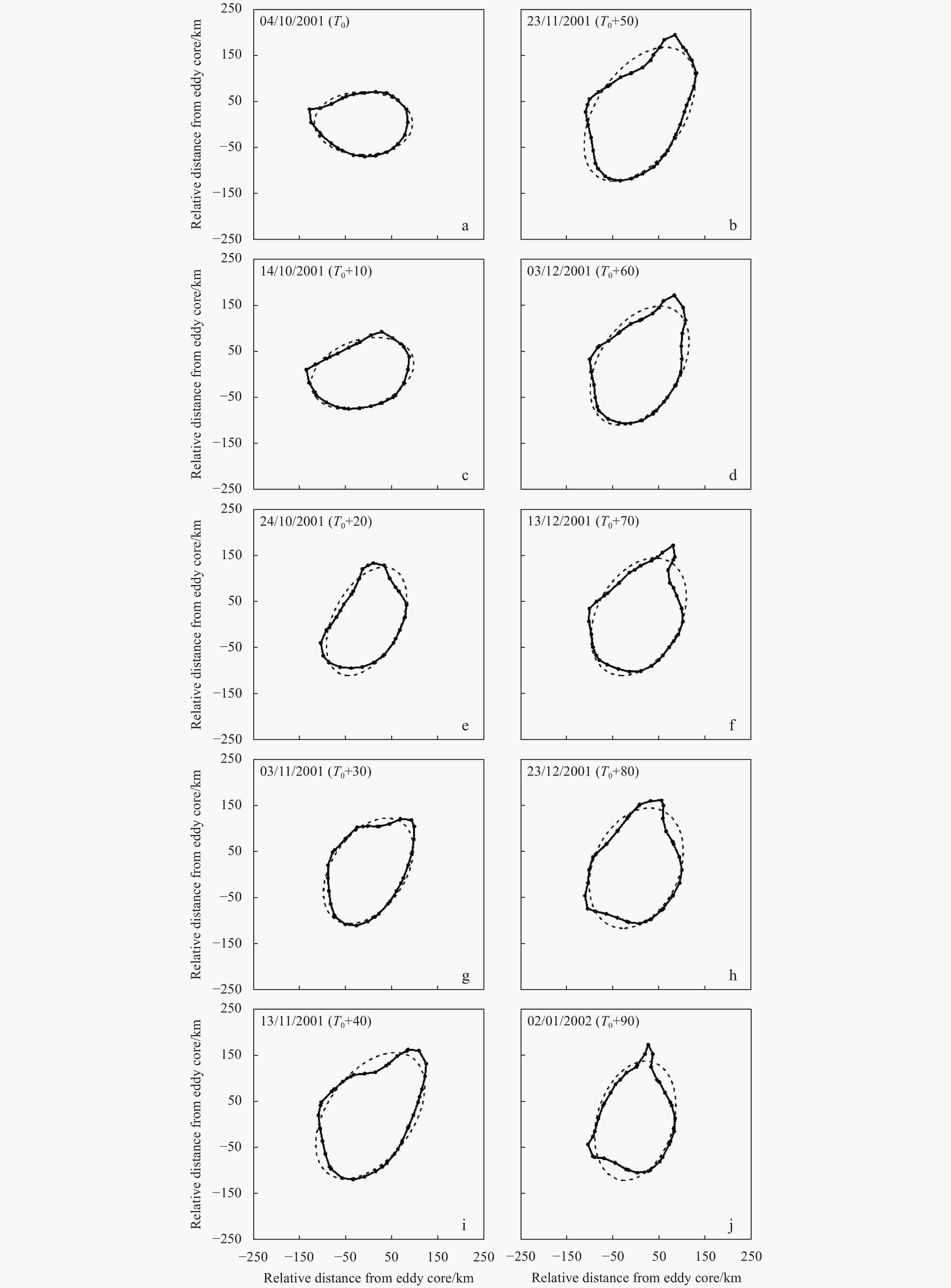
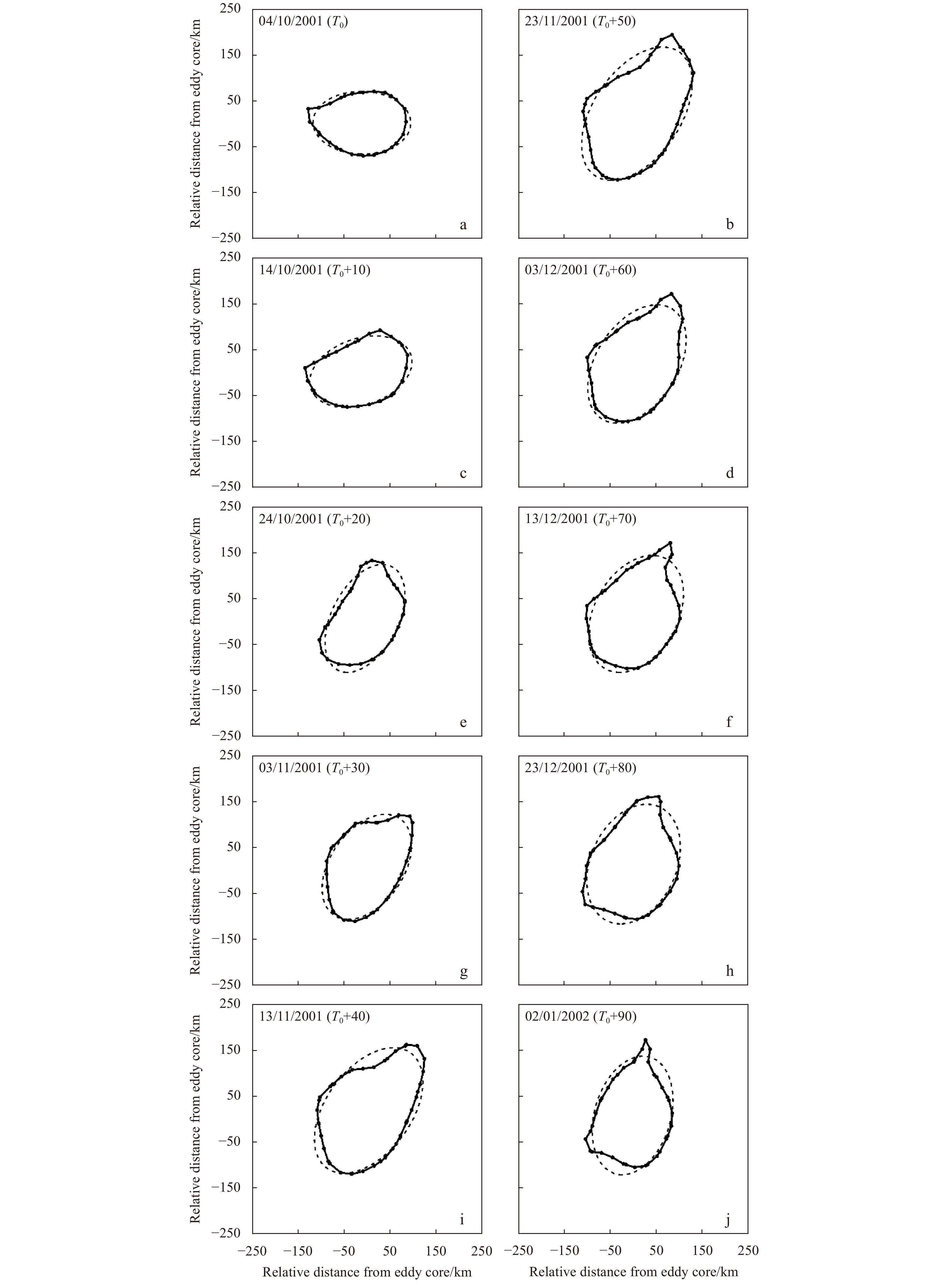
Figure 1. Time series of eddy shape (solid line) for an anticyclonic eddy with a lifetime of 1 641 d in the Pacific Ocean during 4 October 2001−2 January 2002. T0 is the initial day, and the time interval is 10 d. The dashed line in each panel denotes the best-fit ellipse to the eddy boundary.
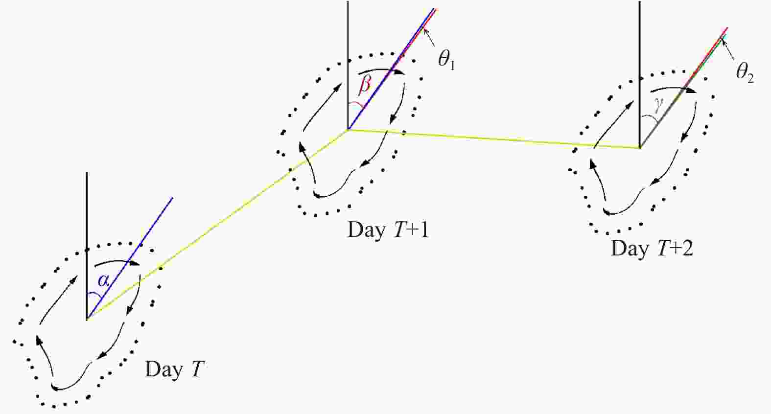
Figure 2. Schematic diagrams of the definition of SOER, internal circulation and migration. ∠θ1=∠β−∠α, ∠θ2=∠γ−∠β.

Figure 3. Flow chart of the algorithm used to extract shape-based overall eddy rotation (SOER) features.
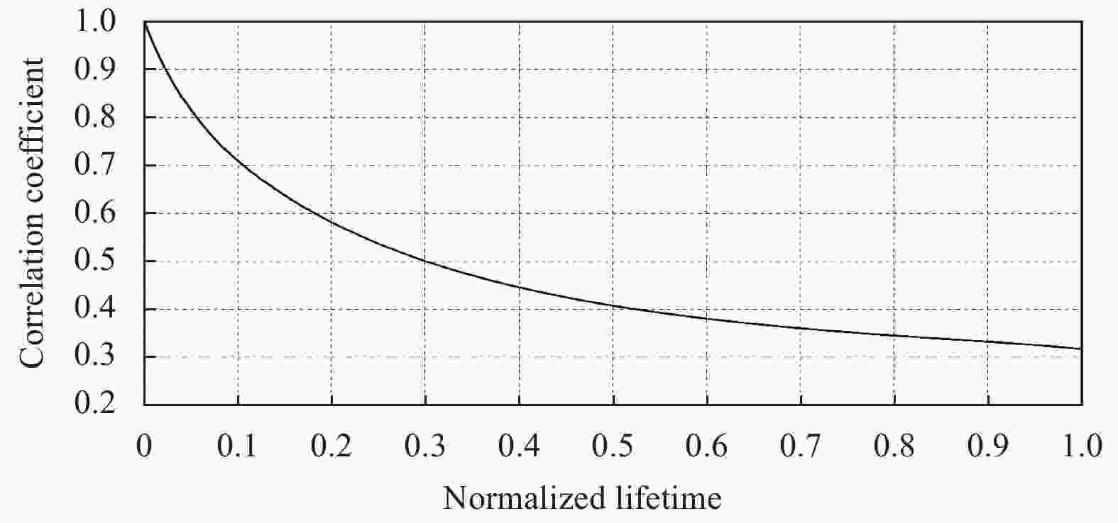
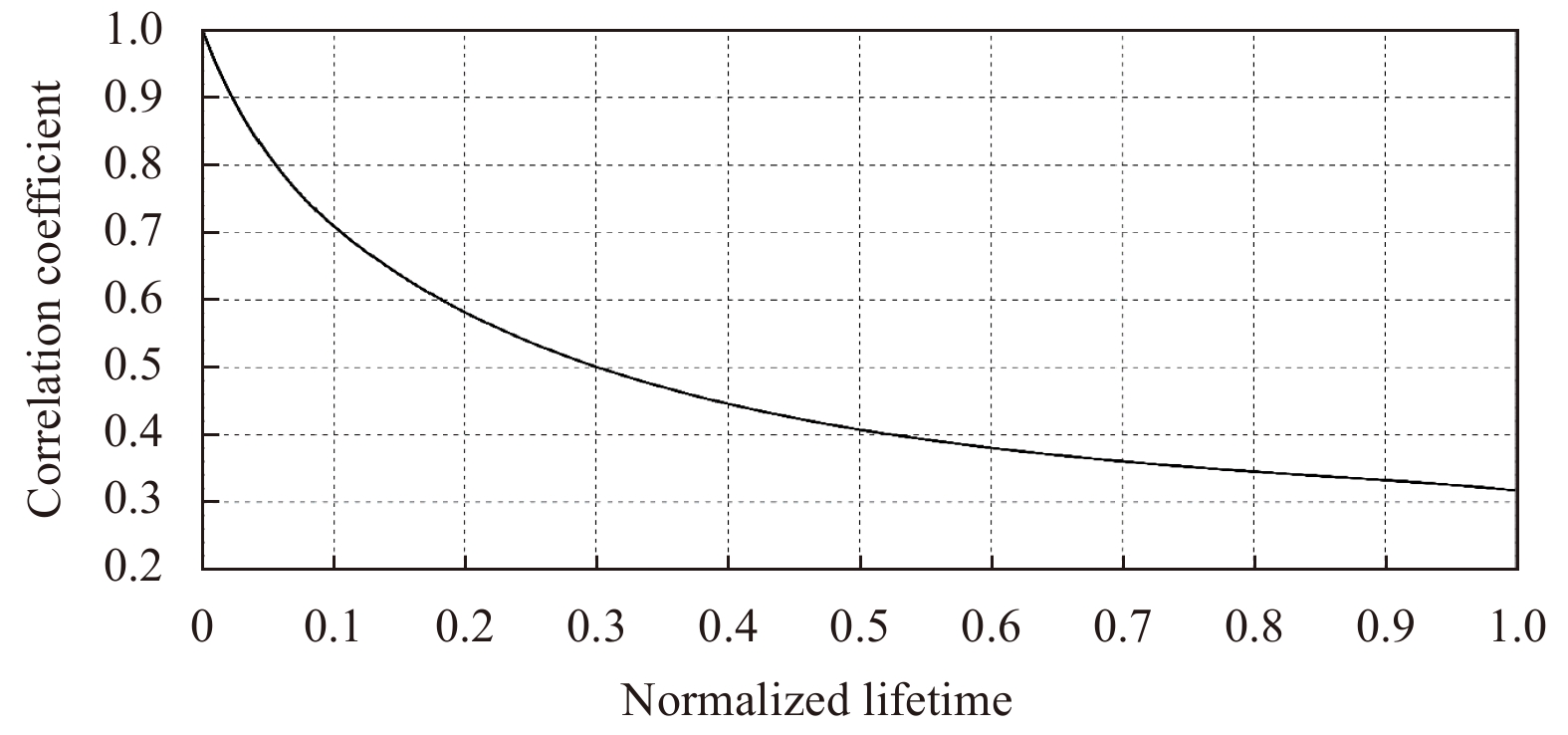
Figure 4. Global mean of the geometric correlation of the eddy shape as a function of normalized lifetime.
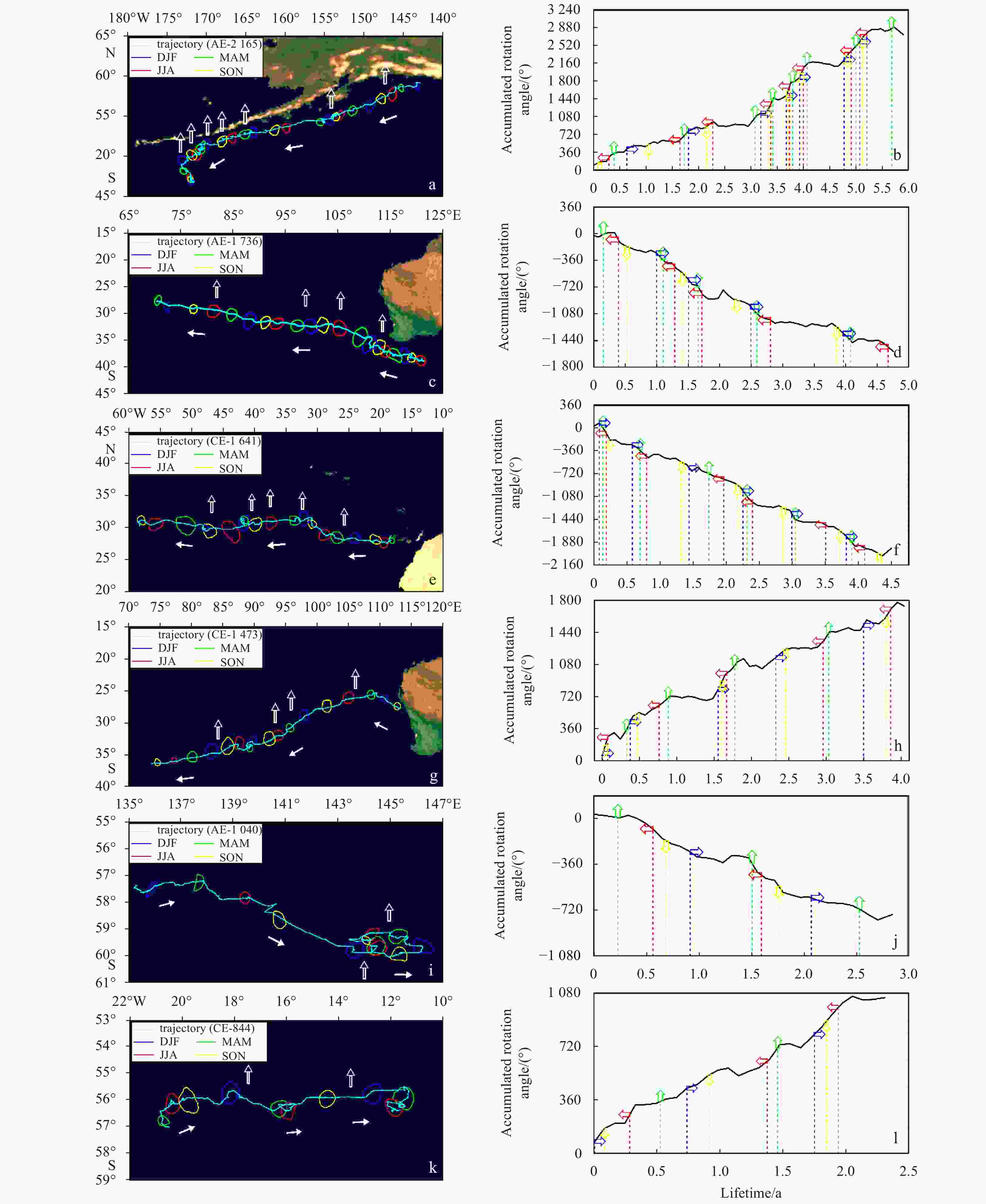
Figure 5. Evolutions of quarterly averaged contours of six LAEs (longest anticyclonic eddies) and LCEs (longest cyclonic eddies) during 1993–2018. a. 6 January 2003–9 December 2008 (2 165 d), c. 6 June 2003–6 March 2008 (1 736 d), e. 19 April 1999–15 October 2003 (1 641 d), g. 8 October 2005–19 October 2009 (1 473 d), i. 3 January 2011–07 November 2013 (1 040 d), and k. 27 April 2012–18 August 2014 (844 d). Blue/DJF, green/MAM, red/JJA and yellow/SON lines represent the periods of December–January–February, March–April–May, June–July–August, and September–October–November, respectively. The light blue curves represent the trajectories of the two eddies, while the solid white arrows indicate their propagation directions. The vertical hollow white arrows indicate the locations where a new overall rotation cycle is started by the eddy orientations. b, d, f, h, j and l. Accumulated angle of the overall rotation of the eddy orientations corresponding to a, c, e, g, i and k, respectively, as represented by the monthly mean orientation of the major axis of the best-fit ellipses. Also overlaid are the timings of the 0°, 90°, 180°, and 270° orientations of the corresponding eddy (the blue, green, red, and yellow vertical dashed lines).

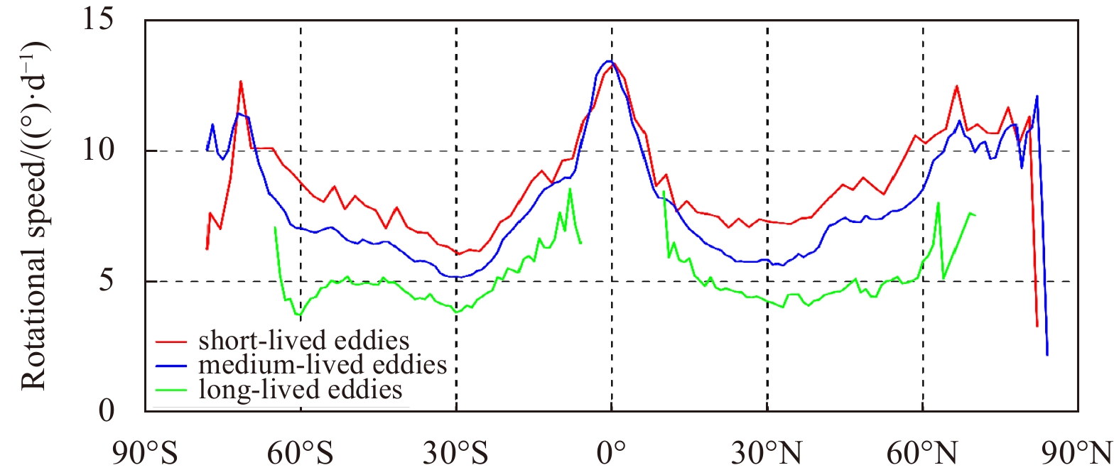
Figure 7. Geographical distribution of rotational speed. EP and WP represent eddies propagating eastward and westward, respectively.
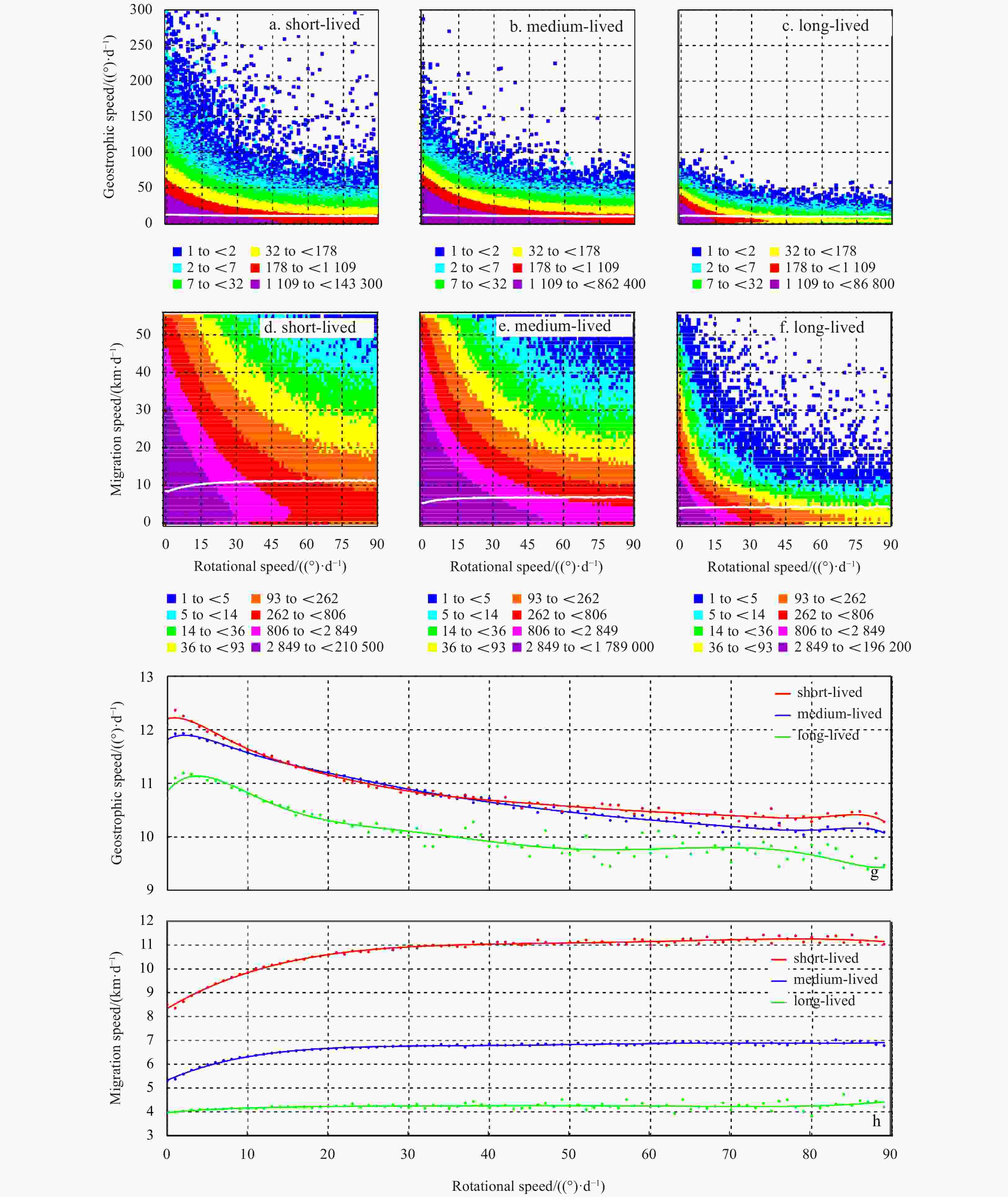
Figure 9. Scatter diagrams of eddy circulation speed (a–c) and migration speed (d–f) versus rotational speed during 1993–2018, respectively. An average curve is overlaid on each panel (white line). Panels g and h are the average circulation speed and average migration speed as a function of eddy rotational speed for short-lived, medium-lived and long-lived oceanic eddies, corresponding to each white line in Panels a–h, respectively.
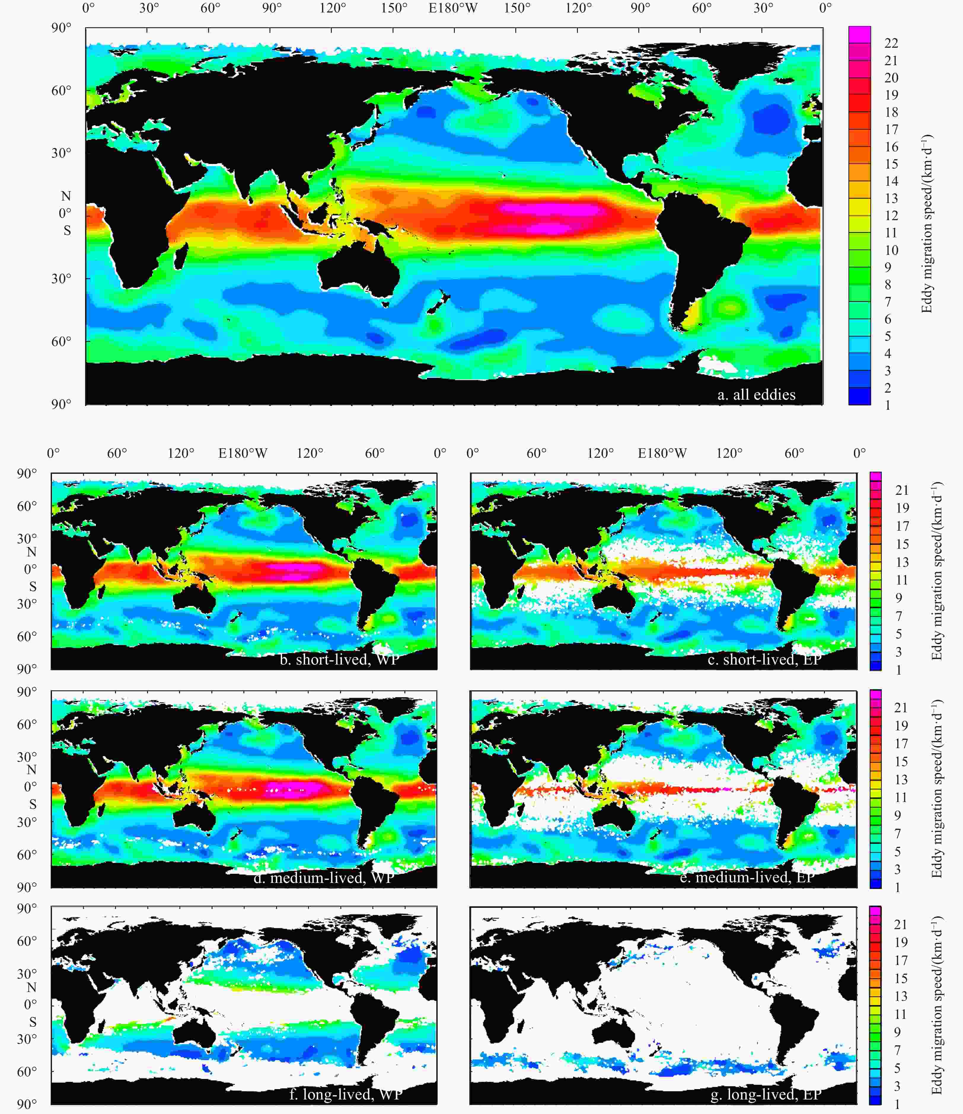
Figure 10. Geographical distribution of eddy migration speed. Note that EP and WP represent eddies propagating eastward and westward, respectively.
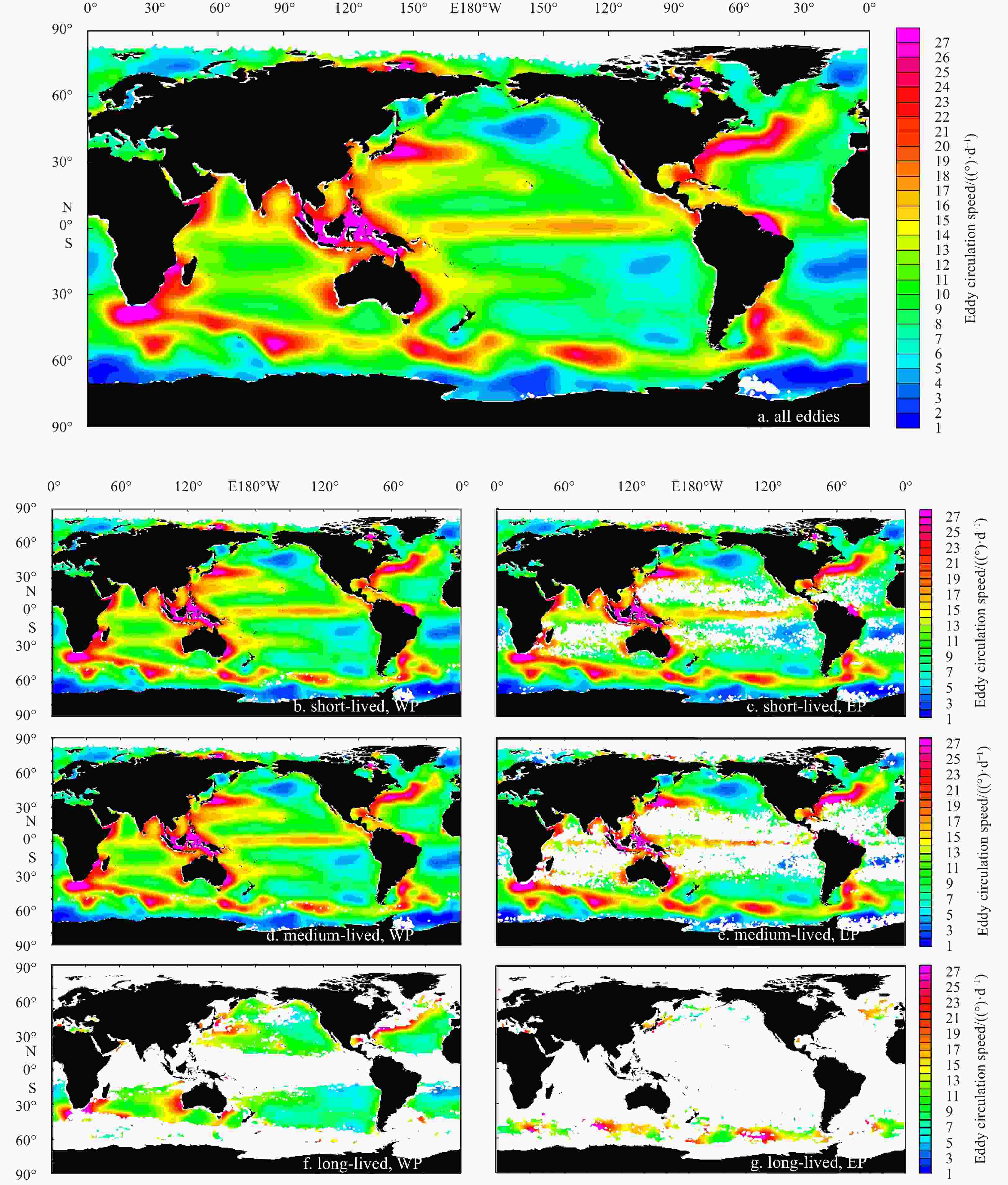
Figure 11. Geographical distribution of eddy circulation speed. EP and WP represent eddies propagating eastward and westward, respectively.
Table 1. Properties of long-lived eddies in Fig. 5
Correspondhg figure Type Lifetime
/dOriginate Terminate Migration direction Migration
distance/kmFig. 5a AE 2 165 59.1°N, 143°W; 6 Jan. 2003 46.6°N, 172.0°W; 9 Dec. 2008 westward 5 657.5 Fig. 5c AE 1 736 38.4°S, 121.1°E; 6 Jun. 2003 27.7°S, 70.3°E; 6 Mar. 2008 westward 6 662.5 Fig. 5e CE 1 641 28.8°N, 18.2°W; 19 Apr. 1999 30.4°N, 58.3°W; 15 Oct. 2003 westward 6 231.3 Fig. 5g CE 1 473 27.8°S, 113.2°E; 8 Oct. 2005 36.4°S, 73.6°E; 19 Oct. 2009 westward 5 498.8 Fig. 5i AE 1 040 57.4°S, 135.3°E; 3 Jan. 2011 59.4°S, 143.9°E; 7 Nov. 2013 eastward 1 894.3 Fig. 5k CE 844 57.0°S, 20.5°W; 27 Apr. 2012 56.4°S, 12.0°W; 18 Aug. 2014 eastward 1 609.7  下载: 导出CSV
Table 2. Categorized statistics of shape-based overall eddy rotation (SOER) direction by lifetime, polarity and hemisphere
Type Loation Rotating dirction Short-lived eddies Medium-lived eddies Long-lived eddies All eddies Number Percentage/% Number Percentage/% Number Percentage/% Number Percentage/% AE NH CW 113 625 49.57 67 211 57.09 960 87.83 181 796 52.23 ACW 115 596 50.43 50 524 42.91 133 12.17 166 253 47.77 SH CW 134 956 46.96 80 426 40.00 234 12.41 215 616 43.97 ACW 152 426 53.04 120 638 60.00 1 652 87.59 274 716 56.03 CE NH CW 113 489 47.88 53 635 42.81 118 18.15 167 242 46.08 ACW 123 541 52.12 71 638 57.19 532 81.85 195 711 53.92 SH CW 143 609 49.84 120 743 57.74 1 505 83.89 265 857 53.27 ACW 144 543 50.16 88 375 42.26 289 16.11 233 207 46.73 Note: SH, southern hemisphere; NH, northern hemisphere; ACW, anti-clockwise; CW, clockwise.
下载: 导出CSV
Table 3. Categorized statistics of shape-based overall eddy rotation (SOER) direction by lifetime, polarity and propagation direction
Type Propagating
directionRotating
dirctionShort-lived eddies Medium-lived eddies Long-lived eddies All eddies Number Percentage/% Number Percentage/% Number Percentage/% Number Percentage/% AE WP CW 173 062 48.06 107 282 47.09 1 033 39.62 281 377 47.65 ACW 187 031 51.94 120 563 52.91 1 574 60.38 309 168 52.35 EP CW 75 519 48.25 40 355 44.37 161 43.28 116 035 46.82 ACW 80 991 51.75 50 599 55.63 211 56.72 131 801 53.18 CE WP CW 175 997 48.71 121 036 50.83 1 273 64.07 298 306 49.60 ACW 185 301 51.29 117 100 49.17 714 35.93 303 115 50.40 EP CW 81 101 49.49 53 342 55.42 350 76.59 134 793 51.72 ACW 82 783 50.51 42 913 44.58 107 23.41 125 803 48.28 Note: ACW, anti-clockwise; CW, clockwise. EP and WP represent eddies propagating eastward and westward, respectively.
下载: 导出CSV
-
[1] Chelton D B, Gaube P, Schlax M G, et al. 2011a. The influence of nonlinear mesoscale eddies on near-surface oceanic chlorophyll. Science, 334(6054): 328–332. doi: 10.1126/science.1208897 [2] Chelton D B, Schlax M G, Samelson R M. 2011b. Global observations of nonlinear mesoscale eddies. Progress in Oceanography, 91(2): 167–216. doi: 10.1016/j.pocean.2011.01.002 [3] Chelton D B, Schlax M G, Samelson R M, et al. 2007. Global observations of large oceanic eddies. Geophysical Research Letters, 34(15): L15606 [4] Chen Ge, Han Guiyan. 2019. Contrasting short-lived with long-lived mesoscale eddies in the global ocean. Journal of Geophysical Research: Oceans, 124(5): 3149–3167. doi: 10.1029/2019JC014983 [5] Chen Ge, Han Guiyan, Yang Xueqing. 2019. On the intrinsic shape of oceanic eddies derived from satellite altimetry. Remote Sensing of Environment, 228: 75–89. doi: 10.1016/j.rse.2019.04.011 [6] Dong Changming, McWilliams J C, Liu Yu, et al. 2014. Global heat and salt transports by eddy movement. Nature Communications, 5(1): 3294. doi: 10.1038/ncomms4294 [7] Dufau C, Orsztynowicz M, Dibarboure G, et al. 2016. Mesoscale resolution capability of altimetry: present and future. Journal of Geophysical Research: Oceans, 121(7): 4910–4927. doi: 10.1002/2015JC010904 [8] Early J J, Samelson R M, Chelton D B. 2011. The evolution and propagation of quasigeostrophic ocean eddies. Journal of Physical Oceanography, 41(8): 1535–1555. doi: 10.1175/2011JPO4601.1 [9] Faghmous J H, Frenger I, Yao Yuanshun, et al. 2015. A daily global mesoscale ocean eddy dataset from satellite altimetry. Scientific Data, 2(1): 150028. doi: 10.1038/sdata.2015.28 [10] Fernandes A M. 2009. Study on the automatic recognition of oceanic eddies in satellite images by ellipse center detection—the Iberian coast case. IEEE Transactions on Geoscience and Remote Sensing, 47(8): 2478–2491. doi: 10.1109/TGRS.2009.2014155 [11] Frenger I, Gruber N, Knutti R, et al. 2013. Imprint of Southern Ocean eddies on winds, clouds and rainfall. Nature Geoscience, 6(8): 608–612. doi: 10.1038/ngeo1863 [12] Fu L L, Chelton D B, Le Traon P Y, et al. 2010. Eddy dynamics from satellite altimetry. Oceanography, 23(4): 14–25. doi: 10.5670/oceanog.2010.02 [13] Gruber N, Lachkar Z, Frenzel H, et al. 2011. Eddy-induced reduction of biological production in eastern boundary upwelling systems. Nature Geoscience, 4(11): 787–792. doi: 10.1038/ngeo1273 [14] Jayne S R, Marotzke J. 2002. The oceanic eddy heat transport. Journal of Physical Oceanography, 32(12): 3328–3345. doi: 10.1175/1520-0485(2002)032<3328:TOEHT>2.0.CO;2 [15] Le Vu B, Stegner A, Arsouze T. 2018. Angular Momentum Eddy Detection and tracking Algorithm (AMEDA) and its application to coastal eddy formation. Journal of Atmospheric and Oceanic Technology, 35(4): 739–762. doi: 10.1175/JTECH-D-17-0010.1 [16] Liu Yingjie, Chen Ge, Sun Miao, et al. 2016. A parallel SLA-based algorithm for global mesoscale eddy identification. Journal of Atmospheric and Oceanic Technology, 33(12): 2743–2754. doi: 10.1175/JTECH-D-16-0033.1 [17] Mason E, Pascual A, McWilliams J C. 2014. A new sea surface height–based code for oceanic mesoscale eddy tracking. Journal of Atmospheric and Oceanic Technology, 31(5): 1181–1188. doi: 10.1175/JTECH-D-14-00019.1 [18] Sun Miao, Tian Fenglin, Liu Yingjie, et al. 2017. An improved automatic algorithm for global eddy tracking using satellite altimeter data. Remote Sensing, 9(3): 206. doi: 10.3390/rs9030206 [19] Tamarin T, Maddison J R, Heifetz E, et al. 2016. A geometric interpretation of eddy Reynolds stresses in barotropic ocean jets. Journal of Physical Oceanography, 46(8): 2285–2307. doi: 10.1175/JPO-D-15-0139.1 [20] Waterman S, Lilly J M. 2015. Geometric decomposition of eddy feedbacks in barotropic systems. Journal of Physical Oceanography, 45(4): 1009–1024. doi: 10.1175/JPO-D-14-0177.1 [21] Yi Jiawei, Liu Zhang, Du Yunyan, et al. 2014. A Gaussian-surface-based approach to identifying oceanic multi-eddy structures from satellite altimeter datasets. In: Proceedings of the 22nd International Conference on Geoinformatics. Kaohsiung, China: IEEE,1–5 [22] Zhang Zhengguang, Qiu Bo, Klein P, et al. 2019. The influence of geostrophic strain on oceanic ageostrophic motion and surface chlorophyll. Nature Communications, 10(1): 2838. doi: 10.1038/s41467-019-10883-w [23] Zhang Zhengguang, Wang Wei, Qiu Bo. 2014. Oceanic mass transport by mesoscale eddies. Science, 345(6194): 322–324. doi: 10.1126/science.1252418 -


 点击查看大图
计量
- 文章访问数: 200
- HTML全文浏览量: 51
- PDF下载量: 6
- 被引次数: 0

