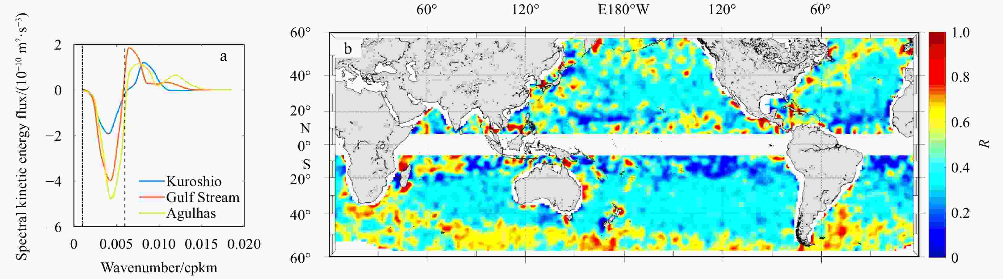
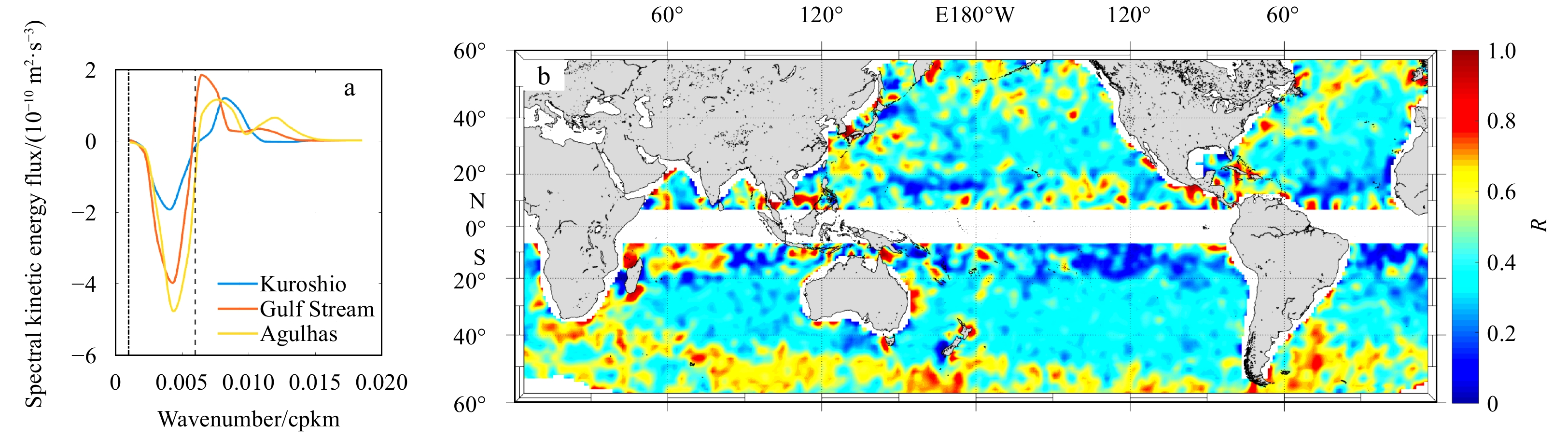
Figure  1.  Time-averaged scalar spectral KE flux versus the wavenumber in the Kuroshio (centered at 35°N, 144°E), the Gulf Stream (centered at 39°N, 64°W), and the Agulhas (centered at 40°S, 19°E) regions (a); and the percentage of the magnitude of the inverse cascade KE relative to that of the total cascade KE (R, b). In a, the vertical dashed line is L_inj, and the vertical dash-dotted line is L_equ. cpkm: cycles per km.

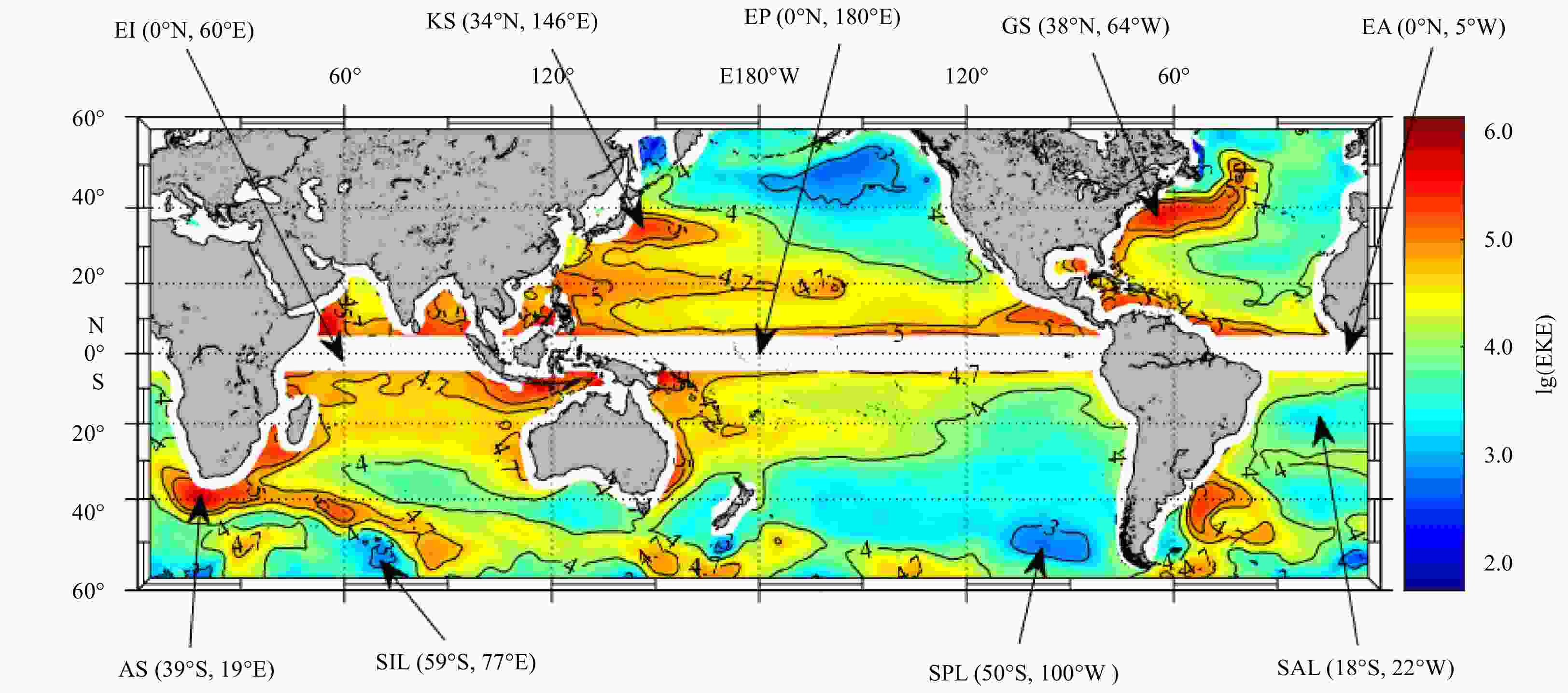
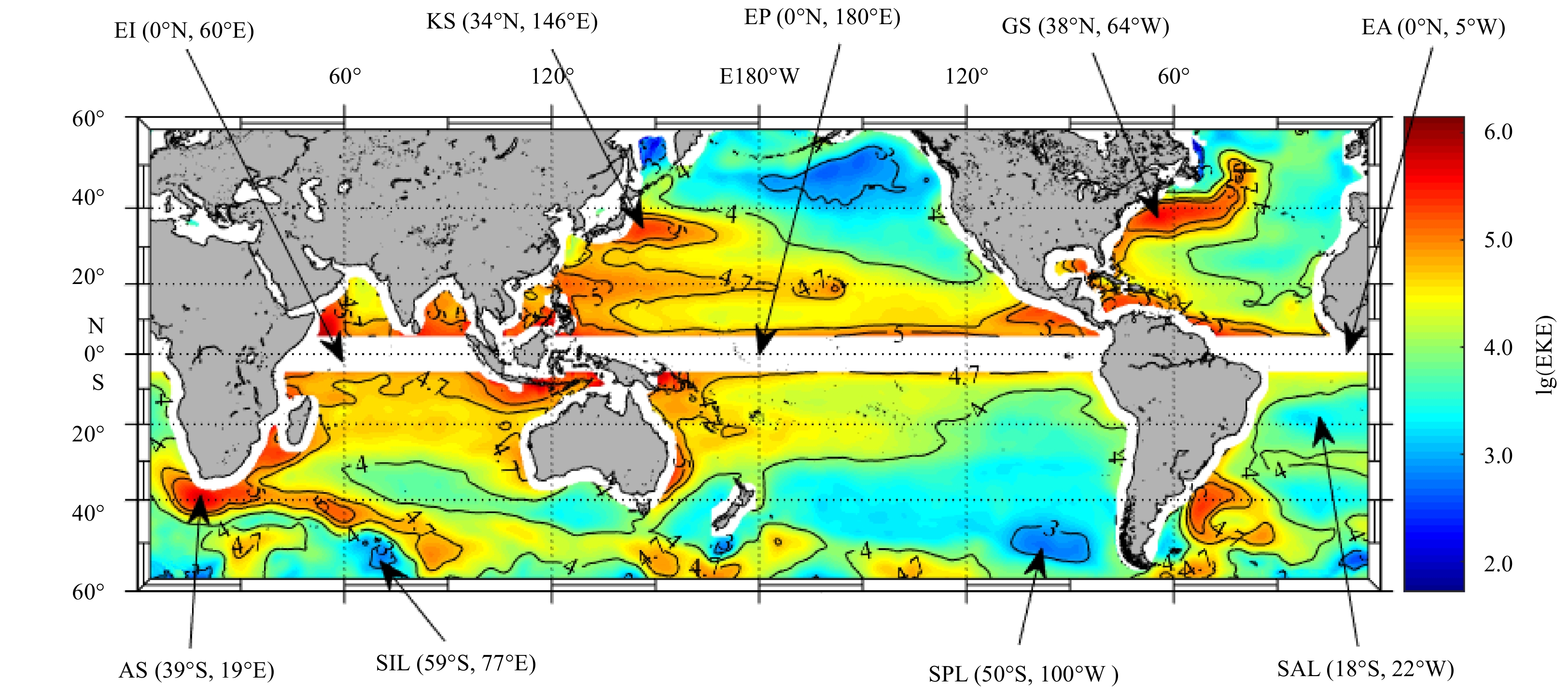
Figure  2.  The global distribution of ${\rm{lg(EKE)}} $. The points marked with arrows are the typical positions selected for subsequent analyses. EI: the equatorial point in the Indian Ocean, KS: Kuroshio, EP: the equatorial point in the Pacific Ocean, GS: Gulf Stream, EA: the equatorial point in the Atlantic Ocean, AS: Agulhas Current, SIL: the low-EKE point in the South Indian Ocean, SPL: the low-EKE point in the South Pacific Ocean, SAL: the low-EKE point in the South Atlantic Ocean.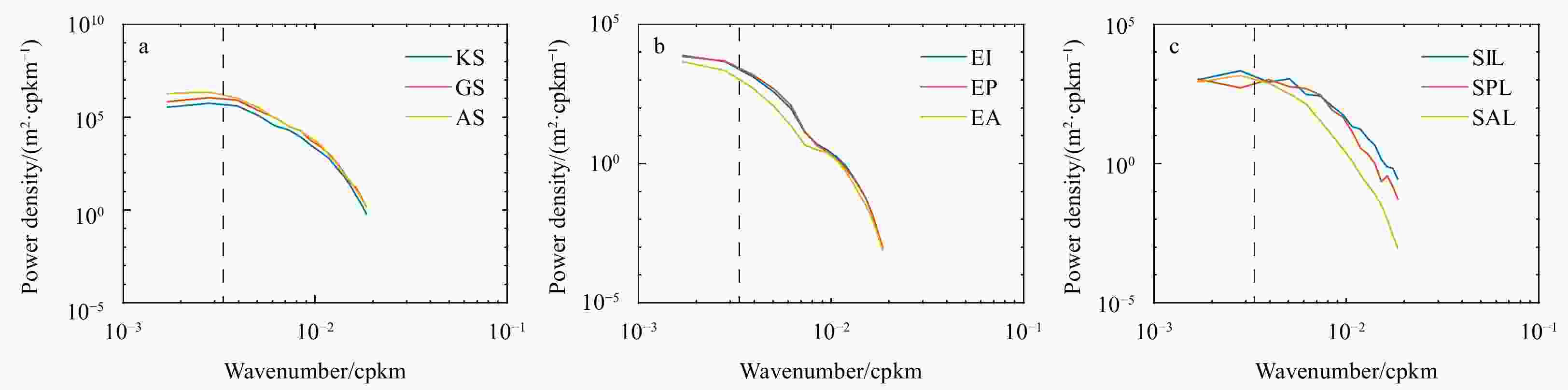

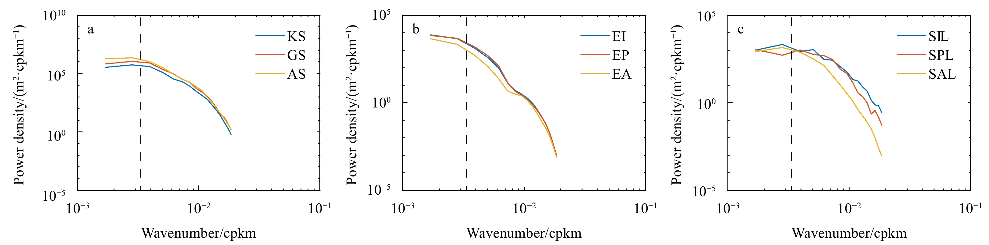
Figure  3.  Time-averaged scalar SSH wavenumber spectrum in high-EKE regions (a), equatorial regions (b), and other low-EKE regions (c). The black dotted line indicates wavelengths of 300 km. KS: Kuroshio, GS: Gulf Stream, AS: Agulhas Current, EI: the equatorial point in the Indian Ocean, EP: the equatorial point in the Pacific Ocean, EA: the equatorial point in the Atlantic Ocean, SIL: the low-EKE point in the South Indian Ocean, SPL: the low-EKE point in the South Pacific Ocean, SAL: the low-EKE point in the South Atlantic Ocean. cpkm: cycles per km.

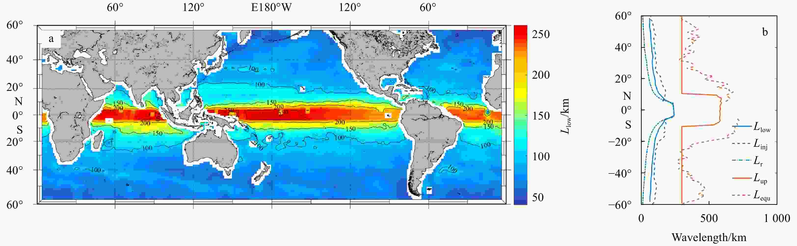
Figure  4.  Spatial distribution of the lower limit (L_low, a) and the zonal average of the lower (blue solid) and upper (orange solid) limits of the variable wavelength range used to fit the spectral slope (b). The Rossby deformation scale L_r (blue dash-dot), the energy injection scale L_inj (blue dash), and the eddy equilibration scale L_equ (orange dash) used to detect the inverse KE cascade band are shown.

Figure  5.  The global distribution of the SSH wavenumber spectral slopes for the inverse KE cascade inertial range. In a, the blue (red) boxes frame the “eddy desert” (subtropical Pacific) regions analyzed in Fig. 6b (Fig. 8); in b, there are three types of areas in terms of the spectral power law. The red color represents regions with spectral slopes following the QG k^11/3 power law within the 95% confidence level, and the blue color represents regions with spectral slopes following the SQG k⁻³ power law. For comparison with the map made by predecessors, the signs of the slopes were reversed to ensure that most values were positive. cpkm: cycles per km.

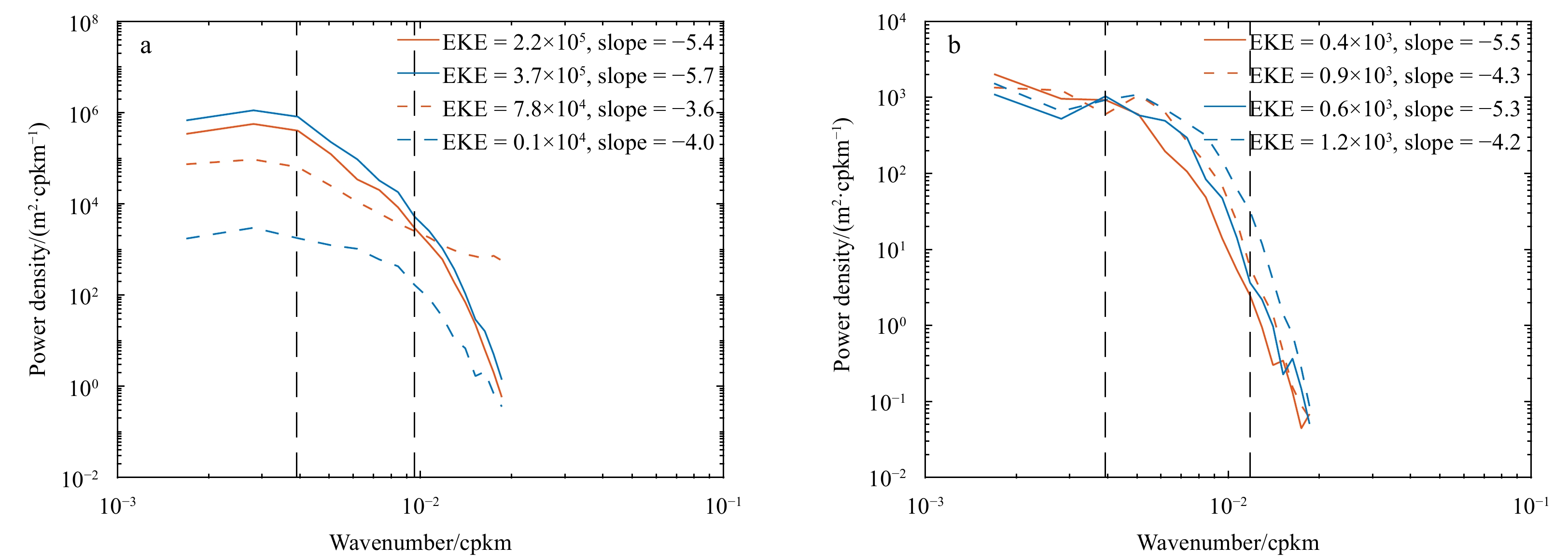
Figure  6.  Time-averaged scalar SSH wavenumber spectra at the Kuroshio centered at (35°N, 146°E) (red solid), the Gulf Stream centered at (39°N, 64°W) (blue solid), the region around the Kuroshio but with a low-EKE level centered at (31°N, 134°E) (red dotted) and the region around the Gulf Stream with a low-EKE level centered at (56°N, 47°W) (blue dotted) (a). Time-averaged scalar SSH wavenumber spectra with the regionally steepest slope (–5.5 and –5.3 respectively) at the “eddy deserts” (marked with blue boxes in Fig. 5a) (solid) and the adjacent regions (dotted). The four regions centered at (48°N, 162°W) (red solid), (42°N, 159°W) (red dotted), (51°S, 101°W) (blue solid), and (46°S, 96°W) (blue solid) (b). The black dotted line indicates the upper and lower limit wavelengths, respectively. cpkm: cycles per km.

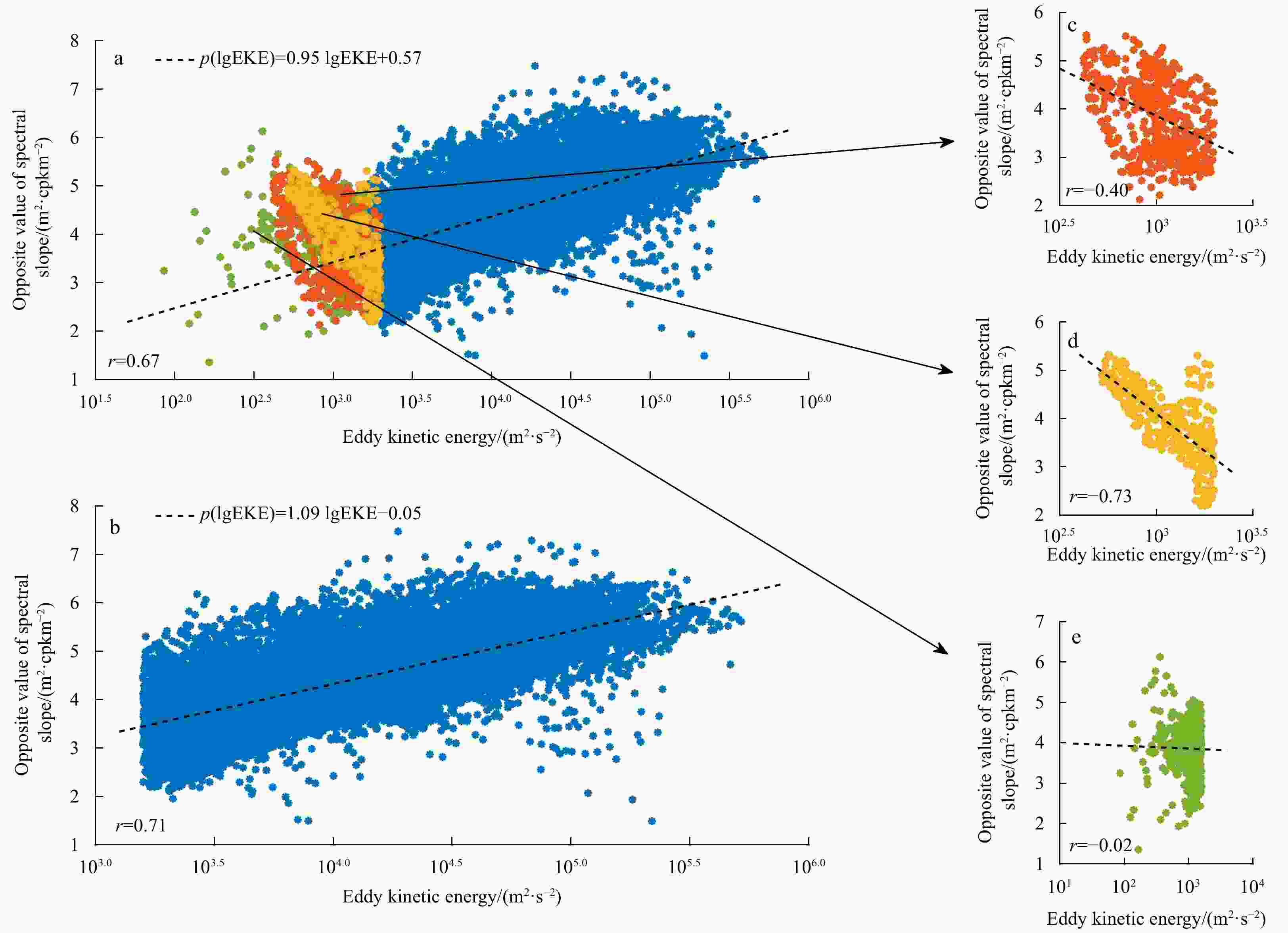
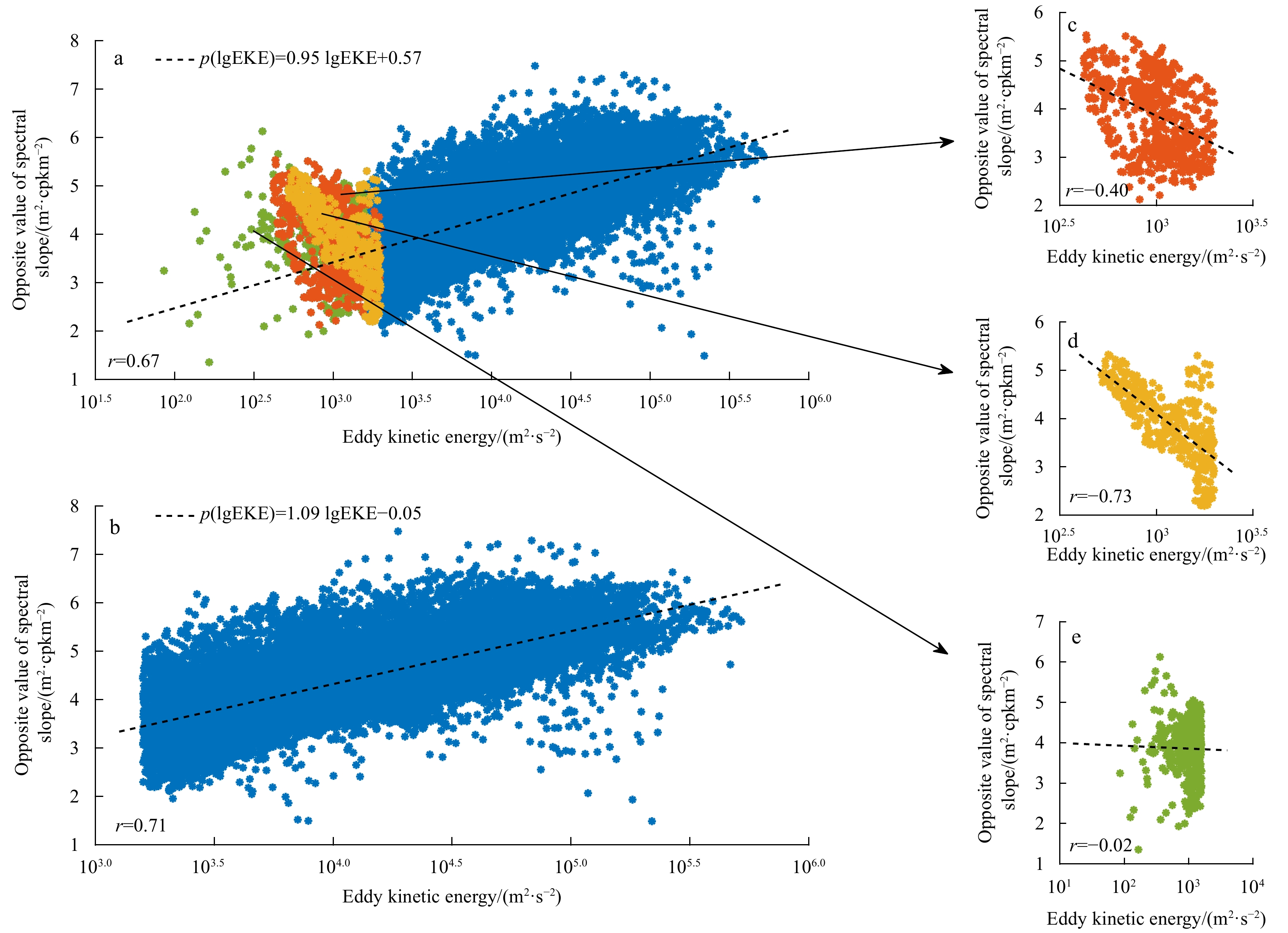
Figure  7.  Scatter diagram between the EKE order of magnitude and the inverse of the wavenumber spectral slope in the global ocean (a), the global ocean without the “eddy deserts” and areas with an EKE lower than 10^3.2 m²/s² (b), the “eddy desert” in the North Pacific (c), the “eddy desert” in the South Pacific (d), and other areas with an EKE lower than 10^3.2 m²/s² (e). The dotted line is the first-order fitting for the scatters. cpkm: cycles per km.

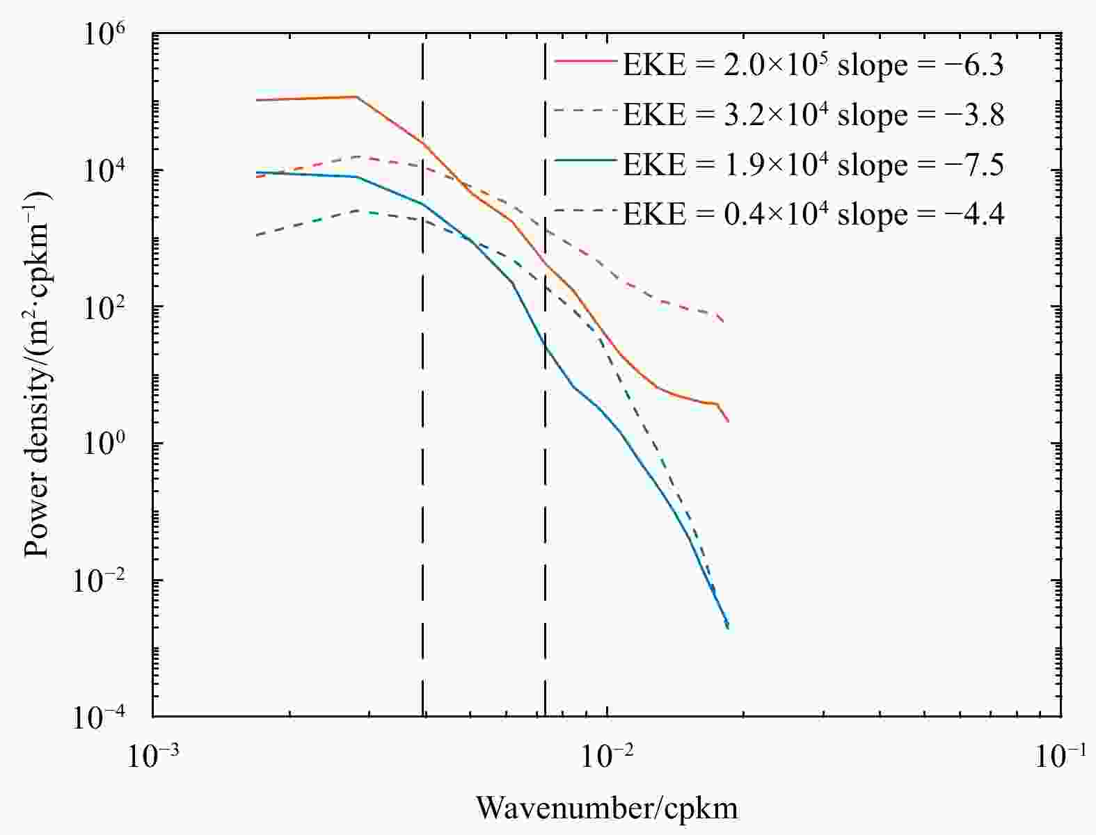
Figure  8.  Time-averaged scalar SSH wavenumber spectra with the steepest slope (–6.3 and –7.5 respectively) in the eastern subtropical Pacific (solid) (framed with red boxes in Fig. 5a) and adjacent regions (dotted). The four regions are centered at (11°N, 93°W) (red solid), (20°N, 109°W) (red dotted), (11°S, 84°E) (blue solid), and (20°S, 100°W) (blue dotted). The black dotted line indicates the upper and lower limit wavelengths. cpkm: cycles per km.

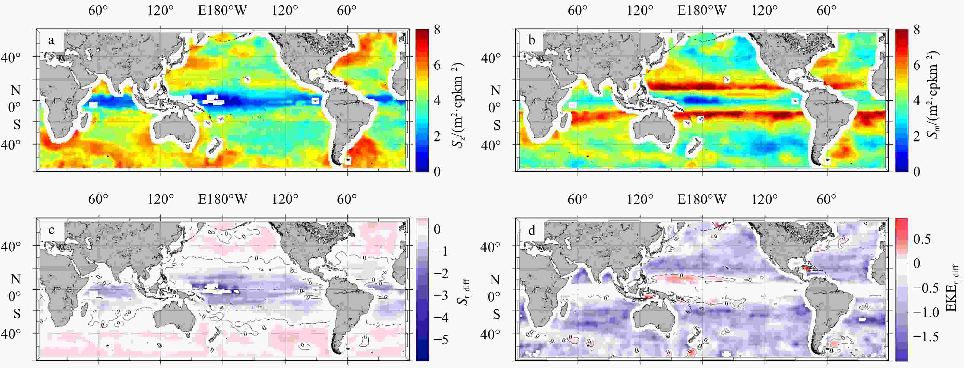
Figure  9.  Zonal (S_z, a), and meridional (S_m, b), SSH wavenumber spectral slopes calculated in the same variable wavelength band as the scalar spectrum, and maps of the relative differences between S_z and S_m (S_{r_diff}, c), as well as relative differences between EKE_z and EKE_m (EKE_{r_diff}, d).

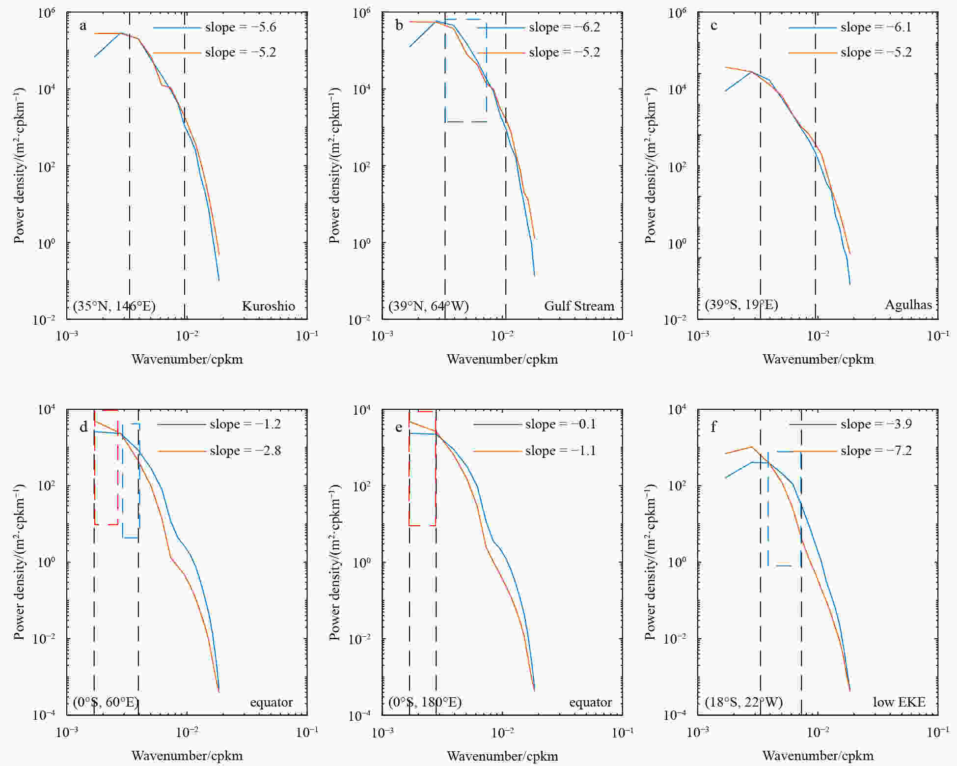
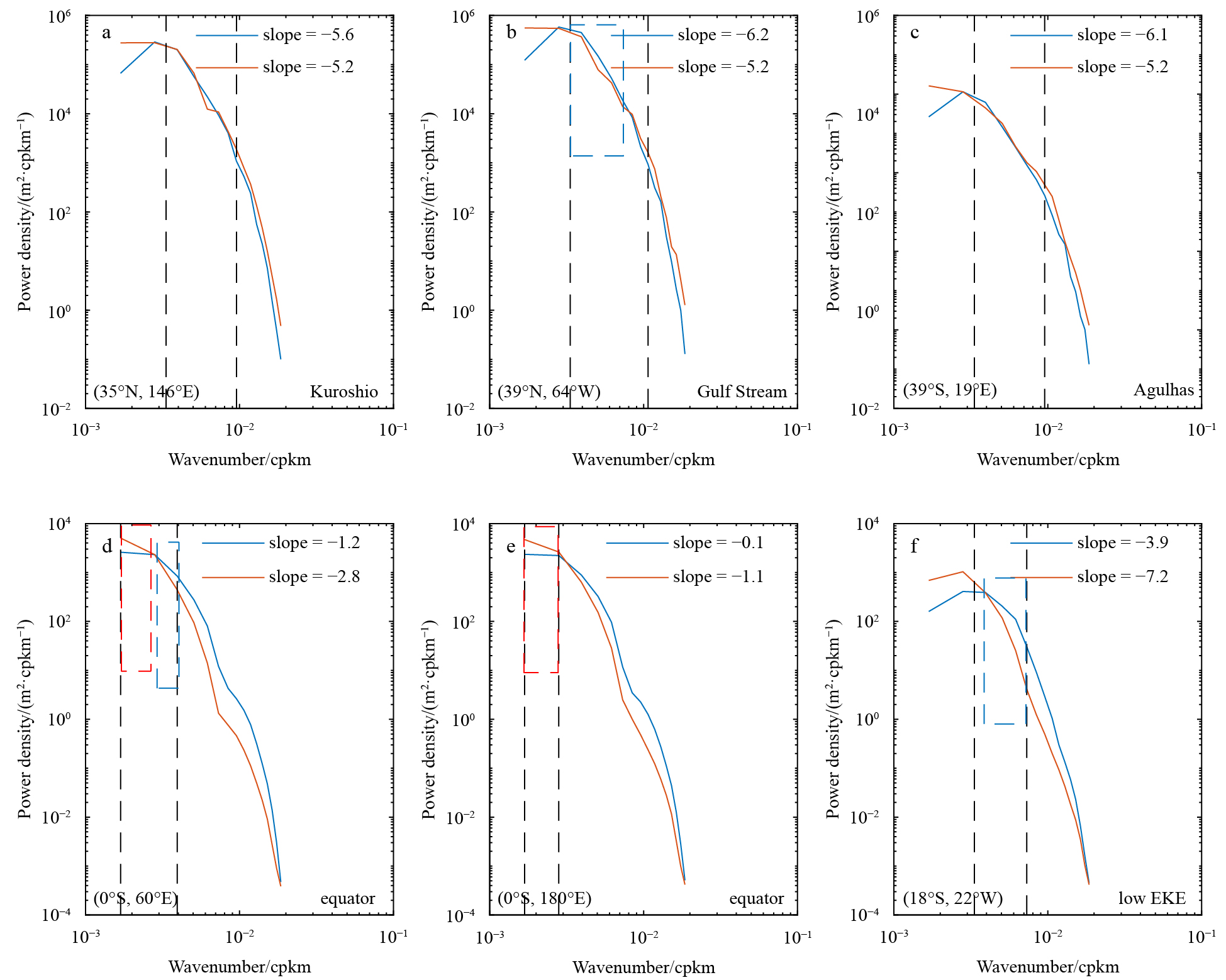
Figure  10.  Zonal (blue) and meridional (red) SSH wavenumber spectra in high-EKE regions (a, b and c), equatorial regions (d and e) and low-EKE regions (f). The black dotted lines indicate the upper and lower limit wavelengths for slope calculation. Obvious anisotropy of the inverse cascade is framed with red (the meridional power density is higher) and blue (the zonal power density is higher) dashed squares.

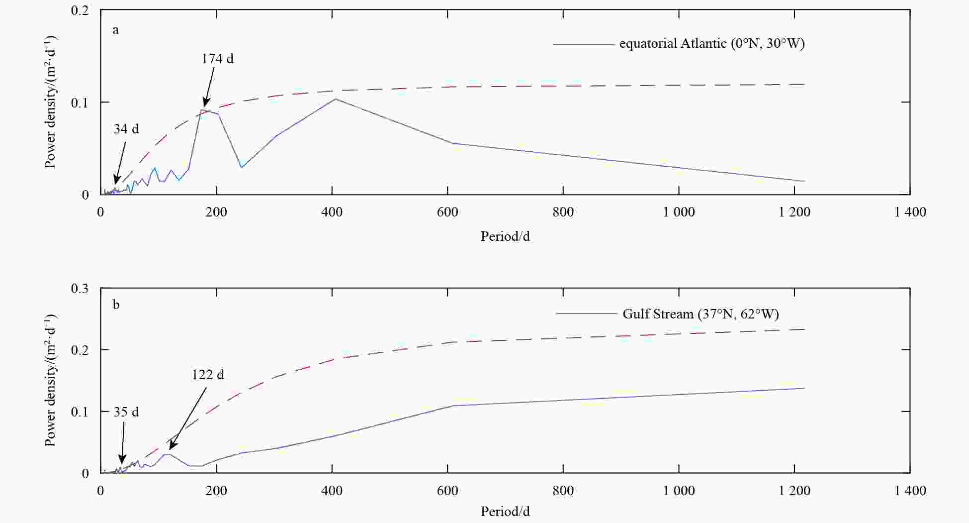
A1.  The power spectra of the regionally averaged (5° × 5°) KE in the equatorial Atlantic (a) and the Gulf Stream (b).

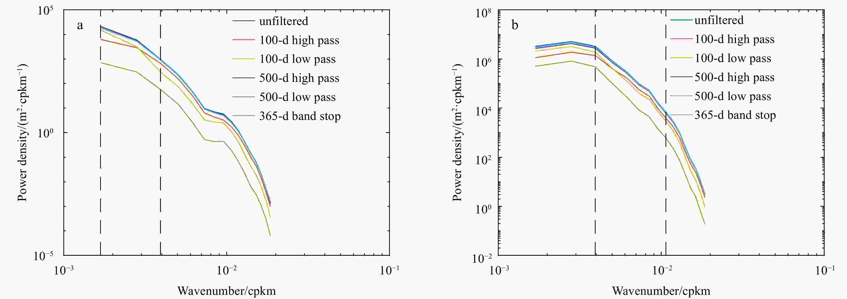
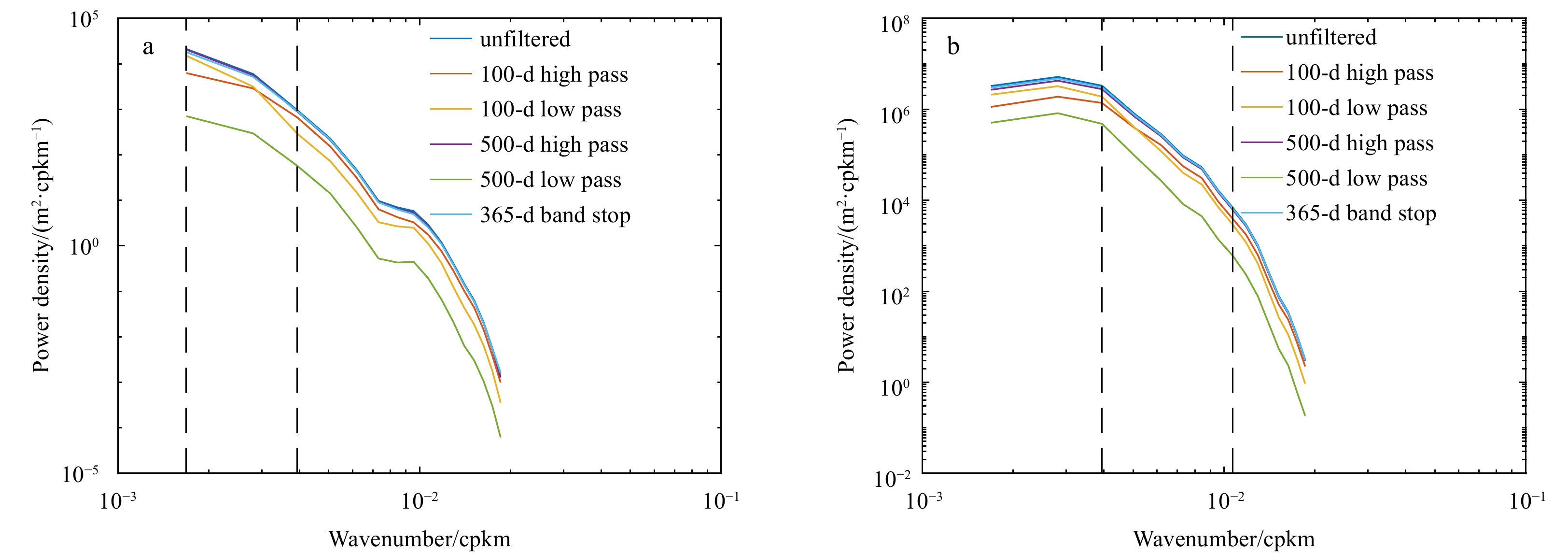
A2.  Time-averaged scalar SSH wavenumber spectra at the equatorial Atlantic Ocean (a) and the Gulf Stream (b) estimated from the data filtered by different methods using 20-a gridded multisatellite measurements. The black dotted lines perpendicular to the x-axis indicate the upper and lower limit wavelengths, respectively.

B1.  The error bar at the 95% confidence level of the spectral slopes of the SSH wavenumber spectrum in the variable wavelength band estimated based on the gridded data from altimeter measurements.