

Application of deep learning technique to the sea surface height prediction in the South China Sea
-
Abstract: A deep-learning-based method, called ConvLSTMP3, is developed to predict the sea surface heights (SSHs). ConvLSTMP3 is data-driven by treating the SSH prediction problem as the one of extracting the spatial-temporal features of SSHs, in which the spatial features are “learned” by convolutional operations while the temporal features are tracked by long short term memory (LSTM). Trained by a reanalysis dataset of the South China Sea (SCS), ConvLSTMP3 is applied to the SSH prediction in a region of the SCS east off Vietnam coast featured with eddied and offshore currents in summer. Experimental results show that ConvLSTMP3 achieves a good prediction skill with a mean RMSE of 0.057 m and accuracy of 93.4% averaged over a 15-d prediction period. In particular, ConvLSTMP3 shows a better performance in predicting the temporal evolution of mesoscale eddies in the region than a full-dynamics ocean model. Given the much less computation in the prediction required by ConvLSTMP3, our study suggests that the deep learning technique is very useful and effective in the SSH prediction, and could be an alternative way in the operational prediction for ocean environments in the future.
-

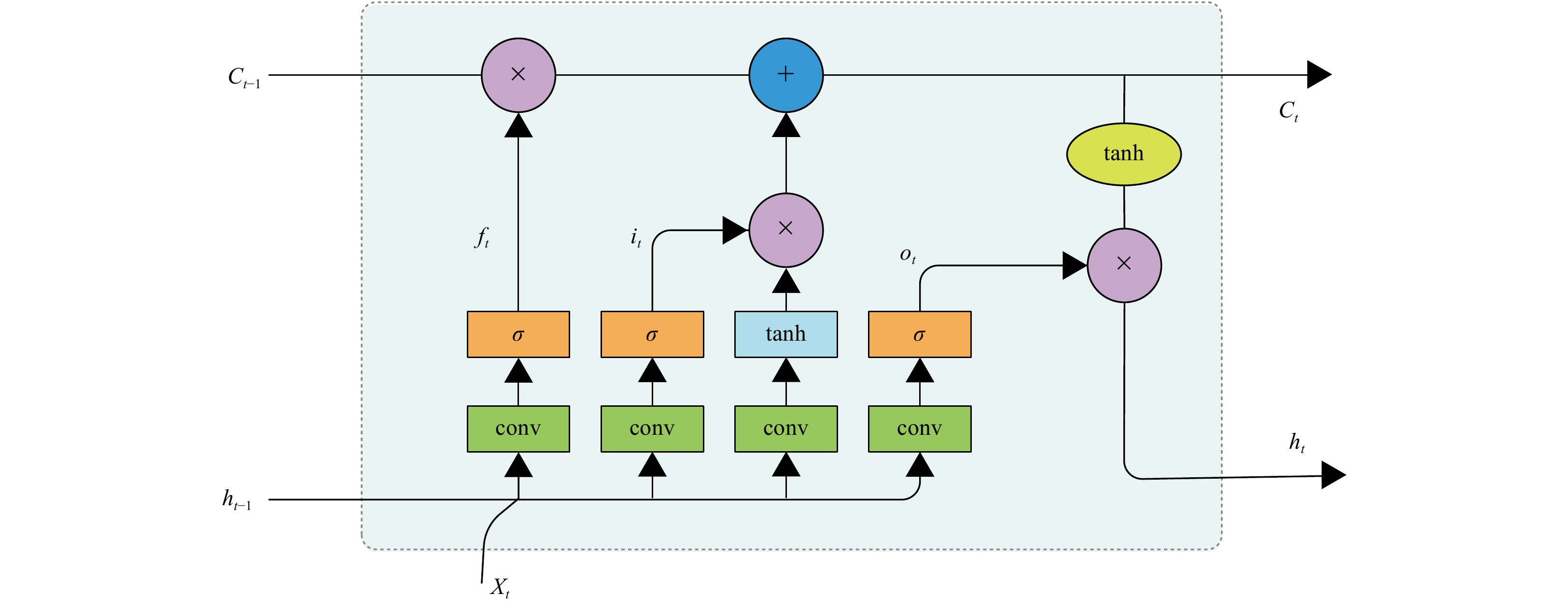
Figure 1. A schematic flow chart of ConvLSTM. “Conv” represents the convolution operation. Spatial information is coded as input in LSTM for tracking temporal evolution. The size of convolutional kenel can be 3×3, 5×5 and 7×7. Multiple kennels are denoted by allows.
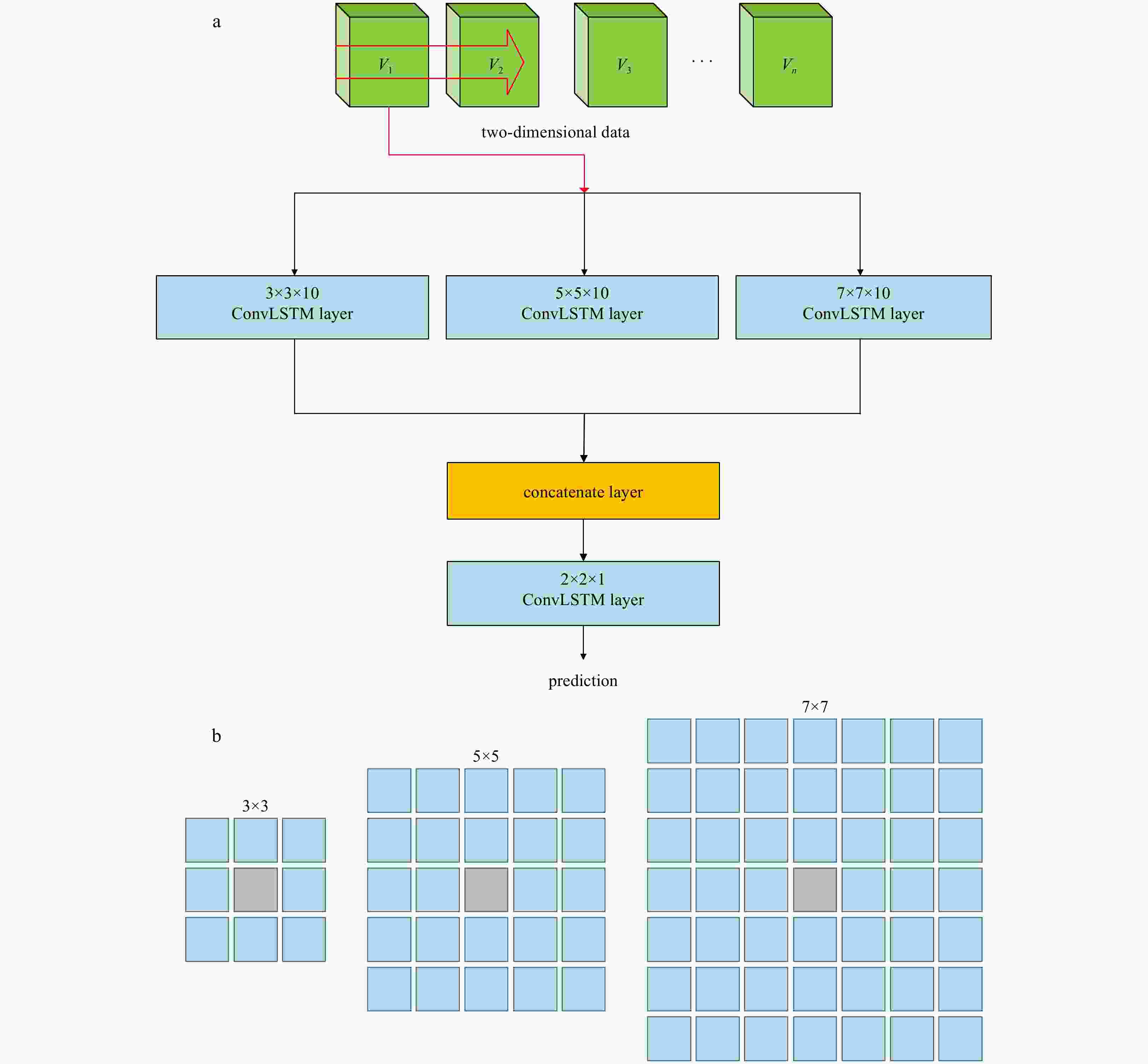
Figure 2. The topologic structure of ConvLSTMP3 (a) and the adjacent grids (blue) of a target grid (gray) corresponding to the convolution kennelsof size 3×3, 5×5, and 7×7 (b). Vi (i=1, 2, …, n) represents datasets that are used to make the i-th-d SSH prediction for a target grid.
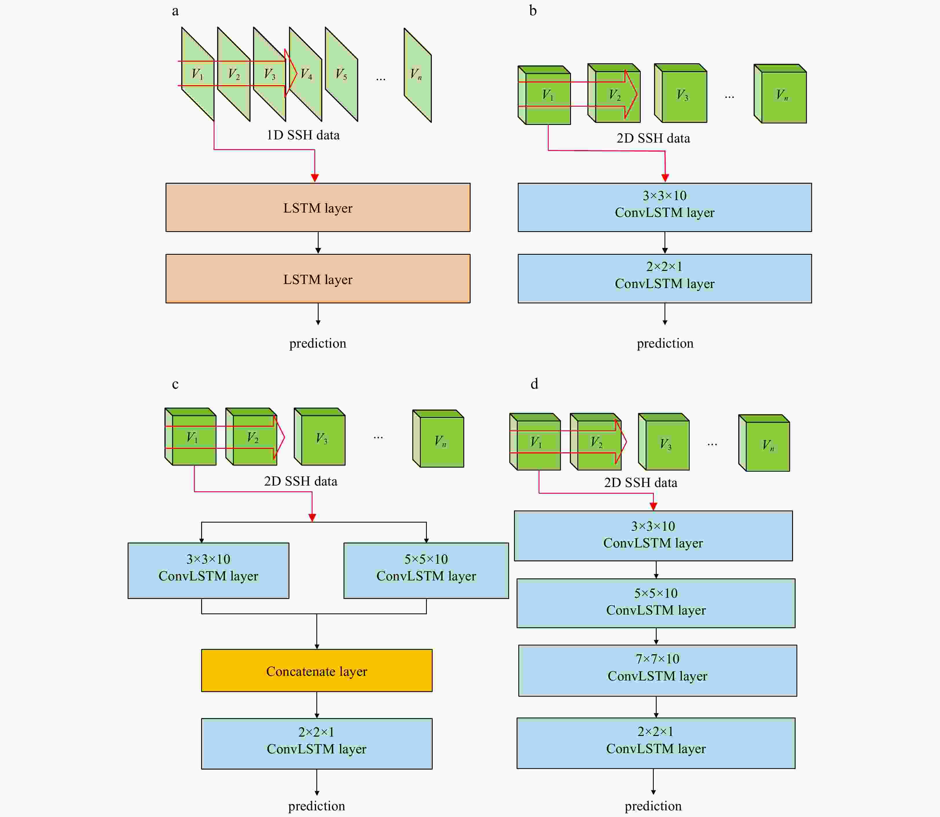
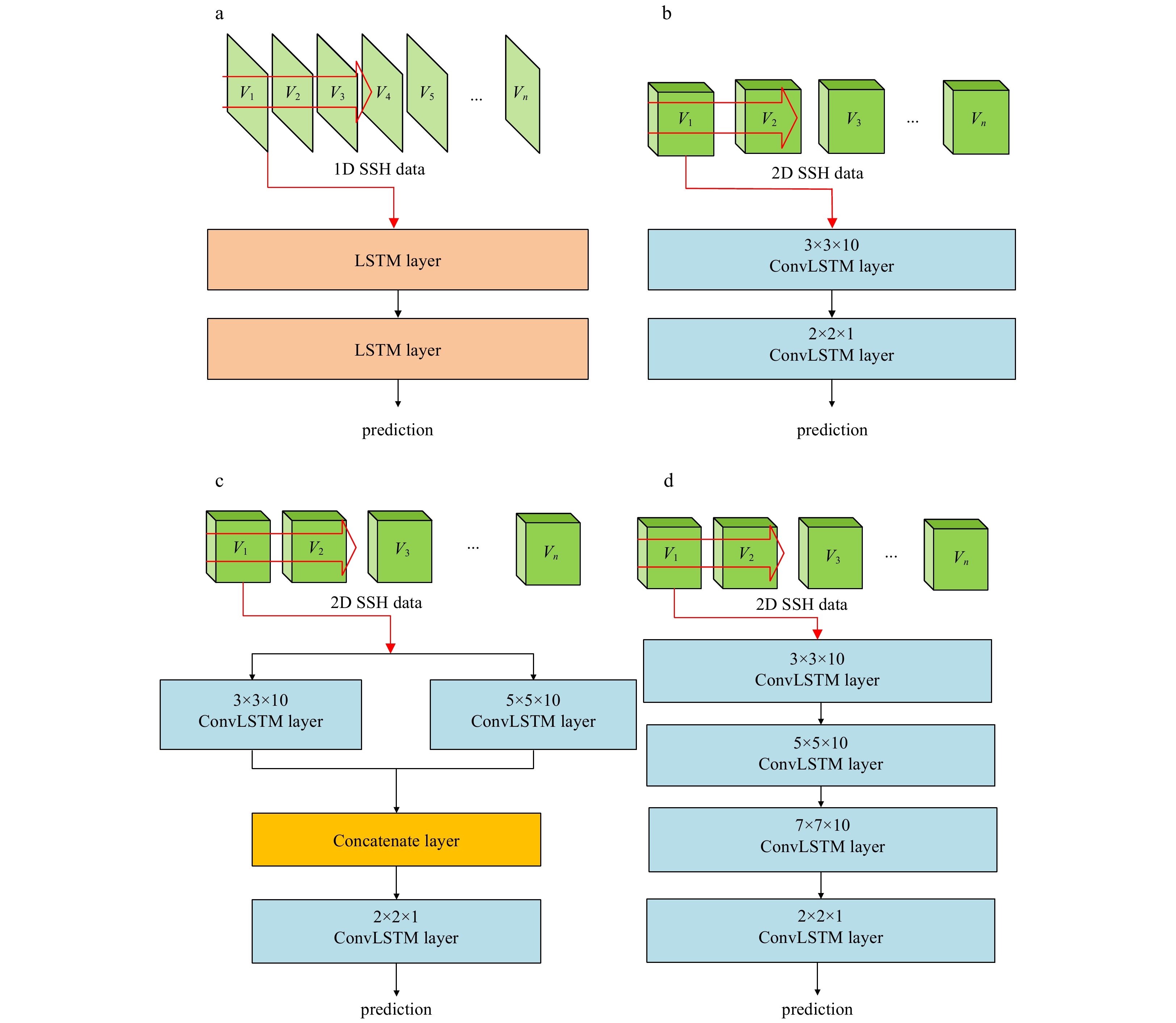
Figure 3. The topologic structures of four models: LSTMS1 (a), ConvLSTMP1 (b), ConvLSTMP2 (c) and ConvLSTMS4 (d). Vi (i=1, 2, …, n) represents datasets that are used to make the i-th-d SSH prediction for a target grid. 1D here means only a time series of SSH data on the target grid, while 2D means multiple time series of SSH data on the target grid as well as its adjacent grids.
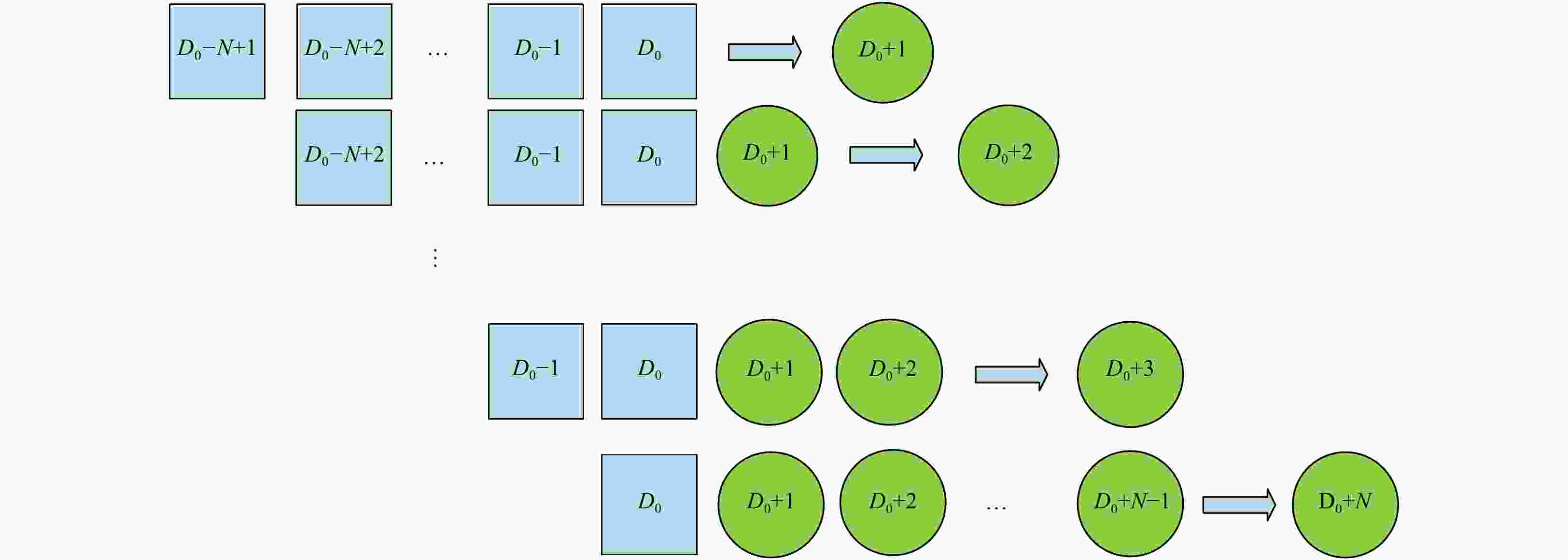
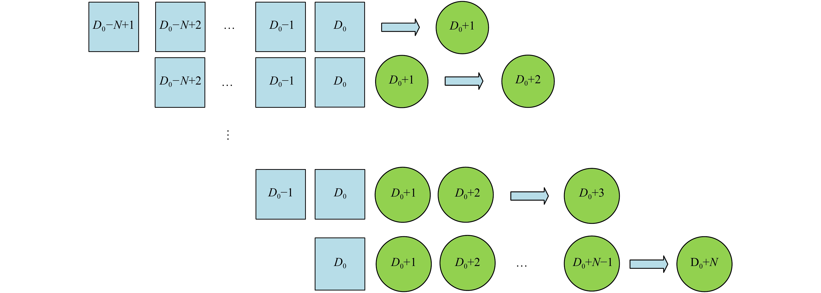
Figure 4. A schematic diagram illustrating a 15-d prediction cycle. The squares and circles represent the historical SSHs and predicted SSHs, respectively. The squares or circles behind the arrows represent the input of ConvLSTMP3 and the circles ahead the arrows represent the output (prediction). D0 denotes the current day of the prediction cycle, and N is the length of prediction cycle which is set to 15 (days).
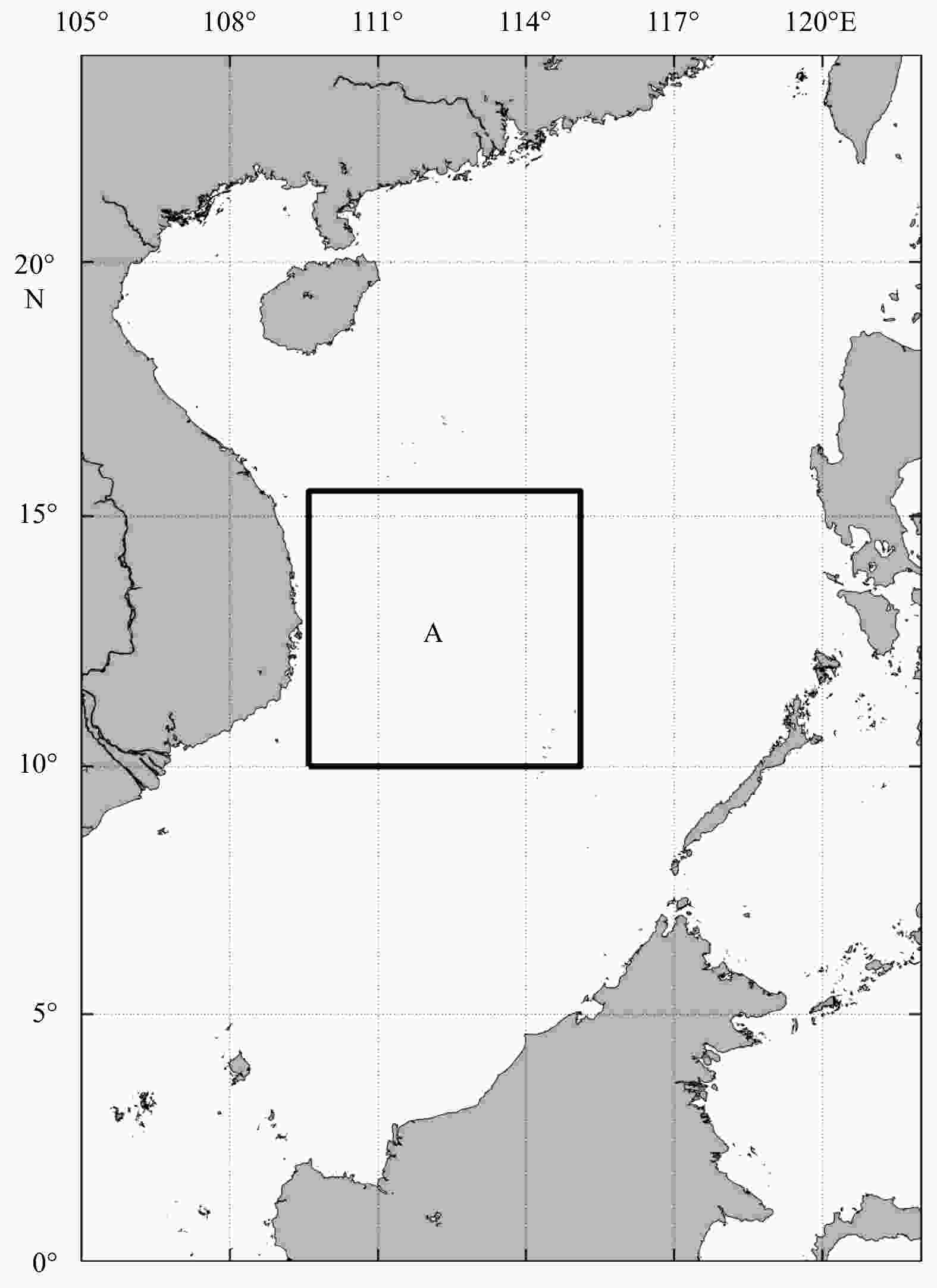
Figure 5. The 5.5°×5.5° region (denoted by A) of the SCS for the deep learning experiments for SSH prediction.
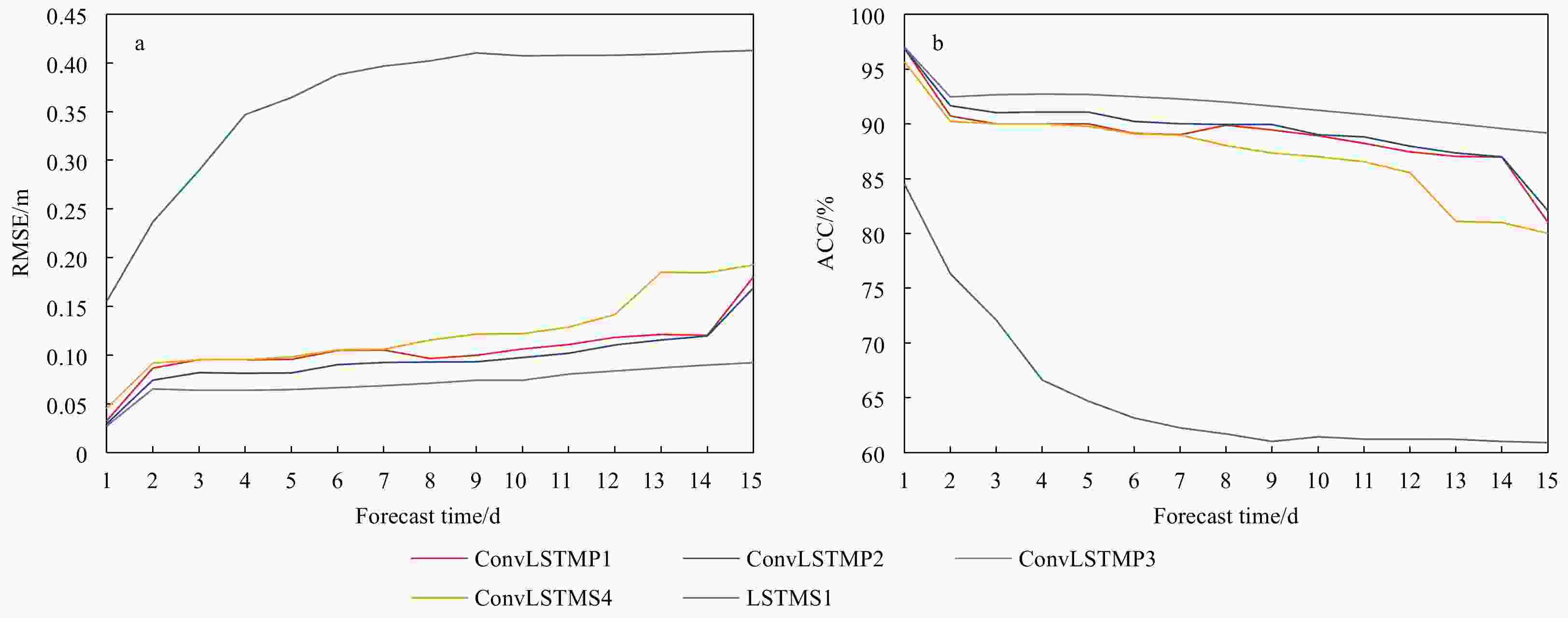
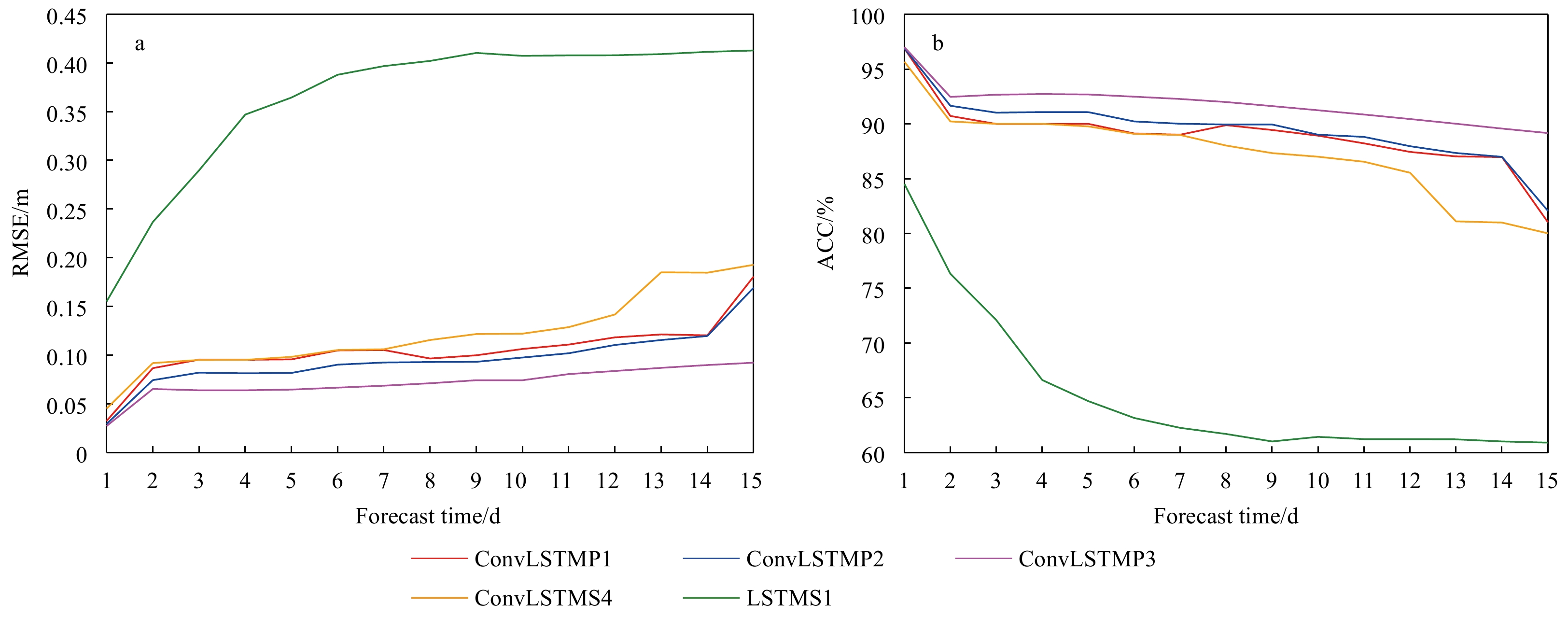
Figure 6. The RMSE and ACC of the 15-d consecutive prediction averaged over the testing period from 6 January 2010 to 31 December 2011 from different schemes.

Figure 7. The ground truth (a–h) and the predicted SSHs by ConvLSTMP3 (i–p) and ROMS (q–x) obtained from August 1 to 15, 2011 in every other day. The black arrows represent the SSH-derived geostrophic currents.
Table 1. The RMSE and ACC of the SSH predictions by ConvLSTMP3 and ROMS during the period of 1–15 August 2011
Period Item RMSE/m ACC/% ConvLSTMP3 ROMS ConvLSTMP3 ROMS Day 1 0.028 0.048 96.4 93.4 Day 2 0.017 0.073 98.0 88.6 Day 3 0.027 0.069 96.2 89.5 Day 4 0.033 0.064 96.3 90.2 Day 5 0.039 0.069 95.0 89.5 Day 6 0.051 0.055 93.0 92.3 Day 7 0.049 0.064 93.9 91.1 Day 8 0.049 0.067 93.8 90.4 Day 9 0.067 0.069 91.6 90.4 Day 10 0.055 0.079 93.5 88.4 Day 11 0.066 0.082 92.2 87.7 Day 12 0.083 0.073 89.4 89.8 Day 13 0.076 0.078 90.3 89.0 Day 14 0.085 0.076 89.5 89.6 Day 15 0.077 0.099 91.3 86.0 15-d mean 0.057 0.072 93.4 89.7  下载: 导出CSV
Table 2. The configurations of the hardware and software as well as the corresponding CPU time used for the 15-d prediction by ConvLSTMP3 and ROMS
Hardware configuration Software configuration CPU time/s ConvLSTMP3 Intel (R) Core (TM) I7-8750H (2.2 GHz) processor, 32 GB memory (total number used: 1) Python 3.6.0 3.695 ROMS Intel (R) Xeon (R) Gold 6132 (2.60 GHz) processor, 125 GB memory (total number used: 112) Mvapich2 2.2b 5.451
下载: 导出CSV
Table 3. The ACC of the SSH predictions by LSTM, GRU, CNN and ConvLSTMP3 during the period of 1–15 August 2011
Periods Item ACC/%
(LSTM)ACC/%
(GRU)ACC/%
(3D CNN)ACC/%
(ConvLSTM)Day 1 84.53 84.77 94.8 96.4 Day 2 76.33 77.33 95.0 98.0 Day 3 72.10 72.20 94.2 96.2 Day 4 66.63 66.67 95.3 96.3 Day 5 64.71 64.71 94.0 95.0 Day 6 63.17 63.23 93.0 93.0 Day 7 62.27 63.01 93.0 93.9 Day 8 61.71 62.00 92.8 93.8 Day 9 61.03 61.07 90.6 91.6 Day 10 61.45 61.55 91.5 93.5 Day 11 61.24 61.43 92.0 92.2 Day 12 61.24 61.24 89.0 89.4 Day 13 61.22 61.21 89.0 90.3 Day 14 61.03 61.05 89.1 89.5 Day 15 60.92 61.00 88.6 91.3 15-d mean 65.30 65.50 92.1 93.4
下载: 导出CSV
-
[1] Braakmann-Folgmann A, Roscher R, Wenzel S, et al. 2017. Sea level anomaly prediction using recurrent neural networks. arXiv preprint arXiv: 1710.07099 [2] Cho K, Van Merriënboer B, Gulcehre C, et al. 2014. Learning phrase representations using RNN encoder-decoder for statistical machine translation. arXiv preprint arXiv: 1406.1078v1, 1724–1734 [3] De Bézenac E, Pajot A, Gallinari P. 2019. Deep learning for physical processes: Incorporating prior scientific knowledge. Journal of Statistical Mechanics: Theory and Experiment, 2019(12): 124009. doi: 10.1088/1742-5468/ab3195 [4] Hochreiter S, Schmidhuber J. 1997. Long short-term memory. Neural Computation, 9(8): 1735–1780. doi: 10.1162/neco.1997.9.8.1735 [5] Huang X J, Shan J J, Vaidya V. 2017. Lung nodule detection in CT using 3d convolutional neural networks. In: 2017 IEEE 14th International Symposium on Biomedical Imaging. Melbourne, VIC, Australia: IEEE, 379–383 [6] Iudicone D, Santoleri R, Marullo S, et al. 1998. Sea level variability and surface eddy statistics in the Mediterranean Sea from TOPEX/POSEIDON data. Journal of Geophysical Research: Oceans, 103(C2): 2995–3011. doi: 10.1029/97JC01577 [7] Jacobs G A, Hogan P J, Whitmer K R. 1999. Effects of eddy variability on the circulation of the Japan/East Sea. Journal of Oceanography, 55(2): 247–256. doi: 10.1023/A:1007898131004 [8] Ji Shuiwang, Xu Wei, Yang Ming, et al. 2013. 3D Convolutional neural networks for human action recognition. IEEE Transactions on Pattern Analysis and Machine Intelligence, 35(1): 221–231. doi: 10.1109/TPAMI.2012.59 [9] Kumar N K, Savitha R, Al Mamun A. 2017. Regional ocean wave height prediction using sequential learning neural networks. Ocean Engineering, 129: 605–612. doi: 10.1016/j.oceaneng.2016.10.033 [10] Ma Xiaolei, Tao Zhimin, Wang Yinhai, et al. 2015. Long short-term memory neural network for traffic speed prediction using remote microwave sensor data. Transportation Research Part C: Emerging Technologies, 54: 187–197. doi: 10.1016/j.trc.2015.03.014 [11] Mason E, Pascual A, McWilliams J C. 2014. A new sea surface height-based code for oceanic mesoscale eddy tracking. Journal of Atmospheric and Oceanic Technology, 31(5): 1181–1188. doi: 10.1175/JTECH-D-14-00019.1 [12] McWilliams J C. 1985. Submesoscale, coherent vortices in the ocean. Reviews of Geophysics, 23(2): 165–182. doi: 10.1029/RG023i002p00165 [13] Morrow R, Coleman R, Church J, et al. 1994. Surface eddy momentum flux and velocity variances in the Southern Ocean from Geosat altimetry. Journal of Physical Oceanography, 24(10): 2050–2071. doi: 10.1175/1520-0485(1994)024<2050:SEMFAV>2.0.CO;2 [14] Reckinger S, Fox-Kemper B, Bachman S, et al. 2014. Anisotropic mesoscale eddy transport in ocean general circulation models. In: 67th Annual Meeting of the Aps Division of Fluid Dynamics. San Francisco, California: Bulletin of the American Physical Society, 59(20): 23–25 [15] Seki M P, Bidigare R R, Lumpkin R, et al. 2001. Mesoscale cyclonic eddies and pelagic fisheries in Hawaiian waters. In: MTS/IEEE Oceans 2001. An Ocean Odyssey. Conference Proceedings. Honolulu, HI, USA: IEEE [16] Shi Xinglian, Chen Zhourong, Wang Hao, et al. 2015. Convolutional LSTM network: A machine learning approach for precipitation nowcasting. In: Proceedings of the 28th International Conference on Neural Information Processing Systems. Cambridge, MA, USA: MIT Press, 802–810 [17] Shin H C, Roth H R, Gao Mingchen, et al. 2016. Deep convolutional neural networks for computer-aided detection: CNN architectures, dataset characteristics and transfer learning. IEEE Transactions on Medical Imaging, 35(5): 1285–1298. doi: 10.1109/TMI.2016.2528162 [18] Song Tao, Wang Zihe, Xie Pengfei, et al. 2020. A novel dual path gated recurrent unit model for sea surface salinity prediction. Journal of Atmospheric and Oceanic Technology, 37(2): 317–325. doi: 10.1175/JTECH-D-19-0168.1 [19] Soong Y S, Hu J H, Ho C R, et al. 1995. Cold-core eddy detected in South China Sea. Eos, Transactions American Geophysical Union, 76(35): 345–347 [20] Szegedy C, Vanhoucke V, Ioffe S, et al. 2016. Rethinking the Inception Architecture for Computer Vision. Las Vegas, NV, USA: IEEE, 2818–2826 [21] Szegedy C, Liu Wei, Jia Yangqing, et al. 2015. Going deeper with convolutions. Proceedings of the IEEE Conference on Computer Vision and Pattern Recognition. Boston, MA, USA: IEEE, 1–9 [22] Wang Liping, Koblinsky C J, Howden S. 2000. Mesoscale variability in the South China Sea from the TOPEX/Poseidon altimetry data. Deep Sea Research Part I: Oceanographic Research Papers, 47(4): 681–708. doi: 10.1016/S0967-0637(99)00068-0 [23] Weiss J B, Grooms I. 2017. Assimilation of ocean sea-surface height observations of mesoscale eddies. Chaos, 27(12): 126803. doi: 10.1063/1.4986088 [24] Yang Fengyu, Feng Tao, Xu Ganyang, et al. 2020. Applied method for water-body segmentation based on mask R-CNN. Journal of Applied Remote Sensing, 14(1): 014502 [25] Zeng Xiangming, Li Yizhen, He Ruoying. 2015. Predictability of the loop current variation and eddy shedding process in the Gulf of Mexico using an artificial neural network approach. Journal of Atmospheric and Oceanic Technology, 32(5): 1098–1111. doi: 10.1175/JTECH-D-14-00176.1 [26] Zeng Xuezhi, Peng Shiqiu, Li Zhijin, et al. 2014. A reanalysis dataset of the South China Sea. Scientific Data, 1: 140052. doi: 10.1038/sdata.2014.52 [27] Zhang Qin, Wang Hui, Dong Junyu, et al. 2017. Prediction of sea surface temperature using long short-term memory. IEEE Geoscience and Remote Sensing Letters, 14(10): 1745–1749. doi: 10.1109/LGRS.2017.2733548 [28] Zhang Zhengguang, Wang Wei, Qiu Bo. 2014a. Oceanic mass transport by mesoscale eddies. Science, 34(6194): 322–324 [29] Zhang Chunhua, Xi Xiaoliang, Liu Songtao, et al. 2014b. A mesoscale eddy detection method of specific intensity and scale from SSH image in the South China Sea and the Northwest Pacific. Science China Earth Sciences, 57(8): 1897–1906. doi: 10.1007/s11430-014-4839-y [30] Zhang Yuanyuan, Zhao Dong, Sun Jiande, et al. 2016. Adaptive convolutional neural network and its application in face recognition. Neural Processing Letters, 43(2): 389–399. doi: 10.1007/s11063-015-9420-y -


 点击查看大图
计量
- 文章访问数: 707
- HTML全文浏览量: 262
- PDF下载量: 43
- 被引次数: 0

