

Evolving a Bayesian network model with information flow for time series interpolation of multiple ocean variables
-
Abstract: Based on Bayesian network (BN) and information flow (IF), a new machine learning-based model named IFBN is put forward to interpolate missing time series of multiple ocean variables. An improved BN structural learning algorithm with IF is designed to mine causal relationships among ocean variables to build network structure. Nondirectional inference mechanism of BN is applied to achieve the synchronous interpolation of multiple missing time series. With the IFBN, all ocean variables are placed in a causal network visually, making full use of information about related variables to fill missing data. More importantly, the synchronous interpolation of multiple variables can avoid model retraining when interpolative objects change. Interpolation experiments show that IFBN has even better interpolation accuracy, effectiveness and stability than existing methods.
-
Key words:
- Bayesian network /
- information flow /
- time series interpolation /
- ocean variables
-
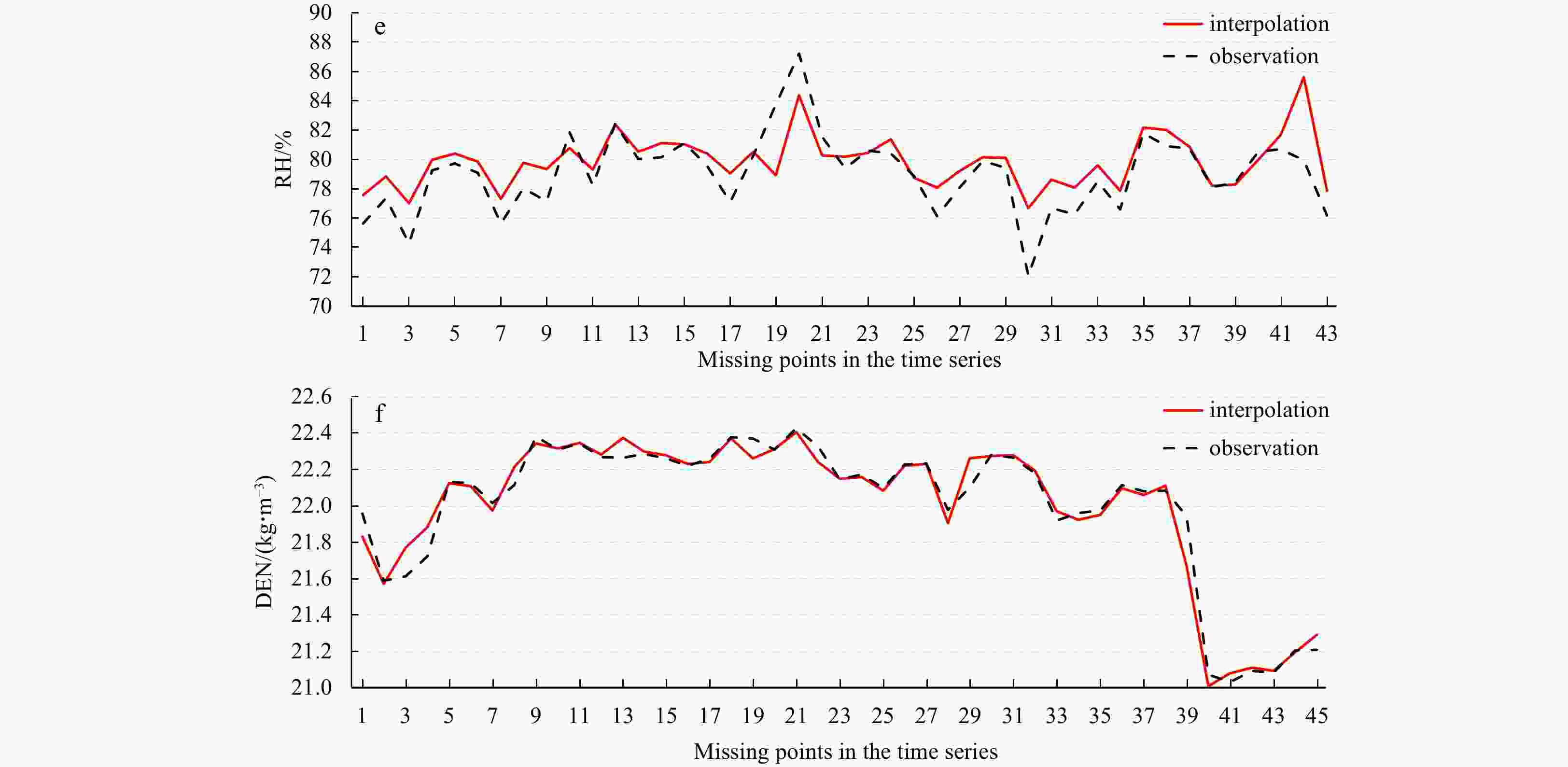
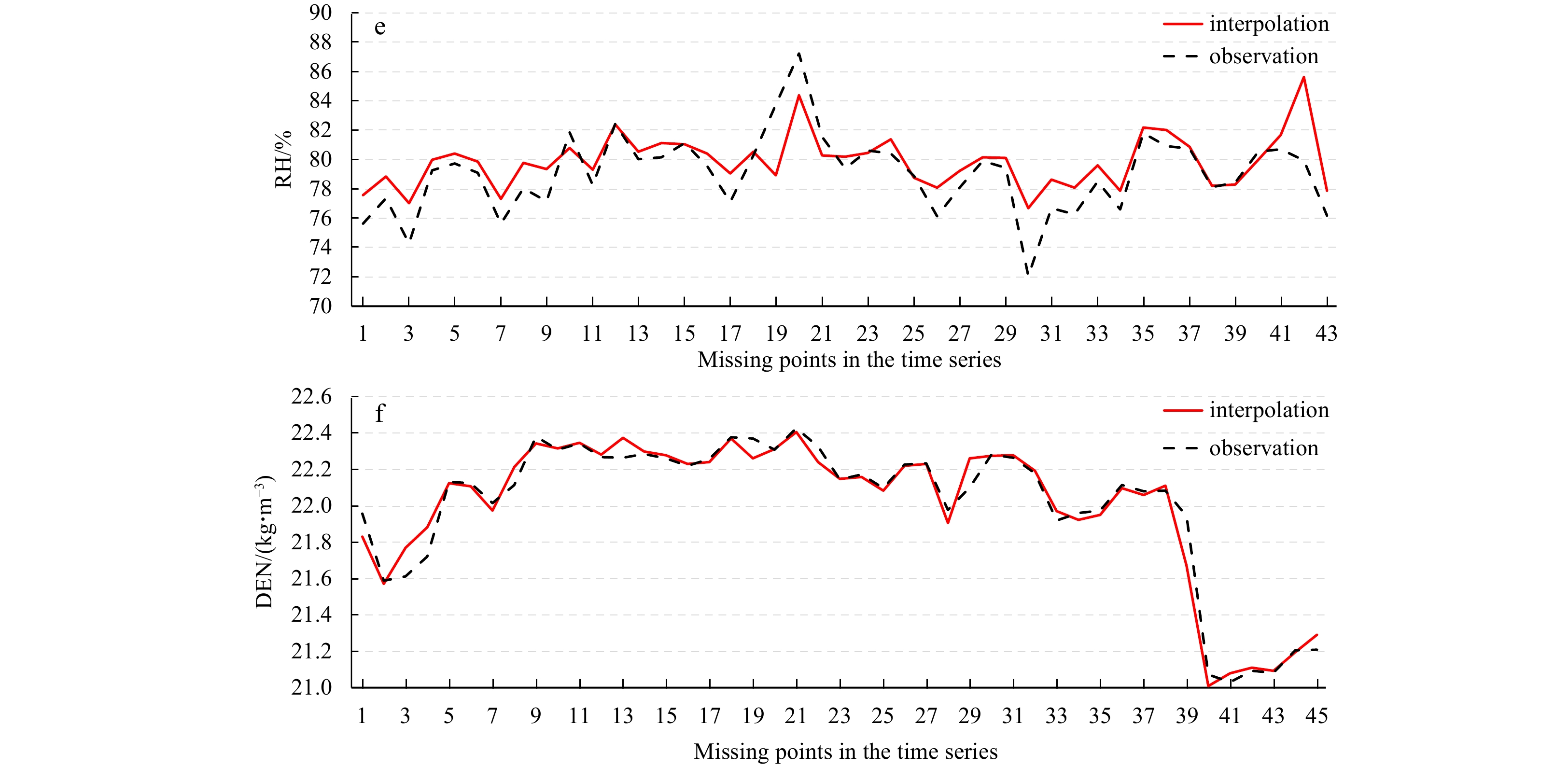
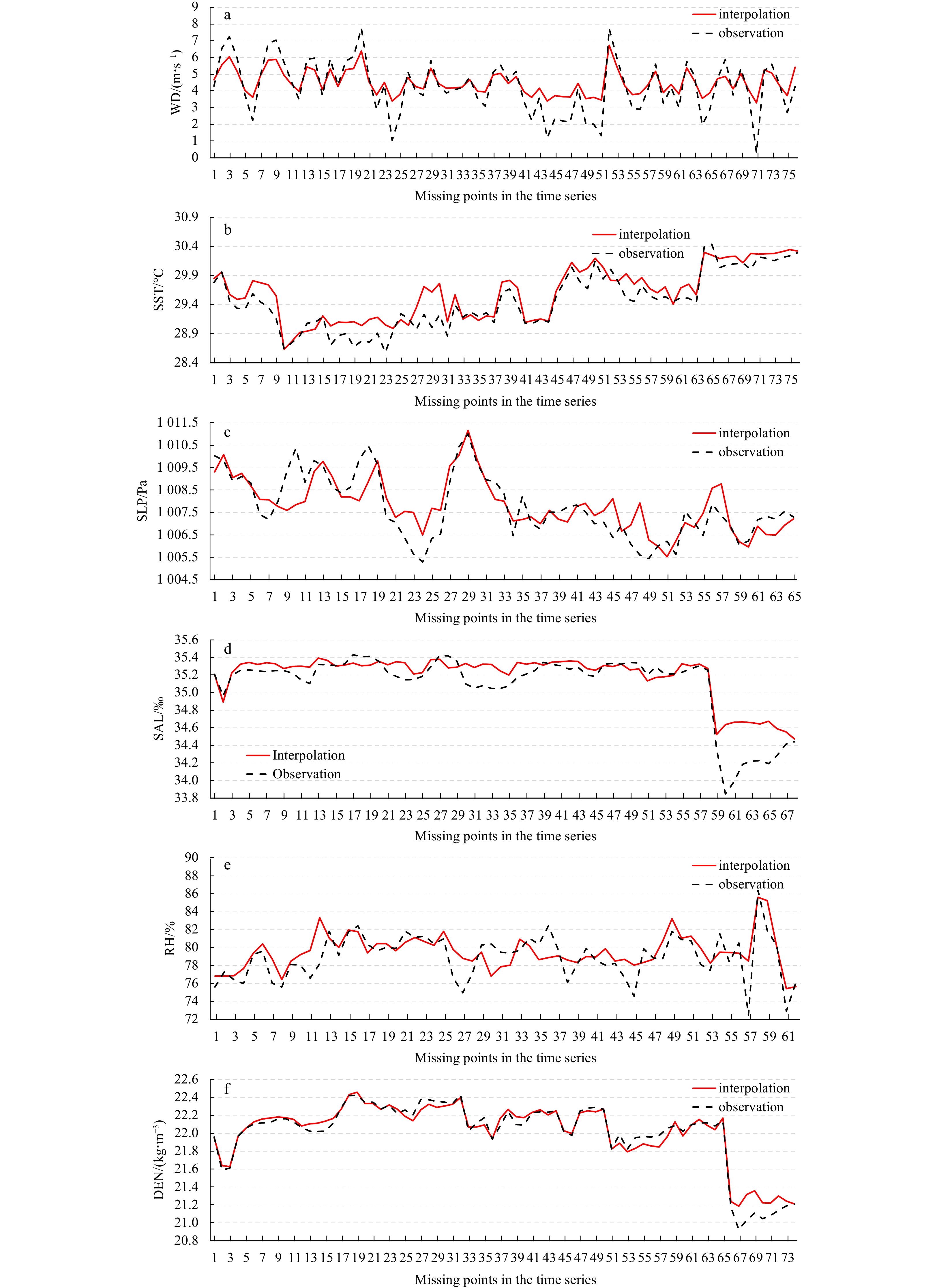
4. Interpolation results with the data missing rate of 40%: WD (a), SST (b), SLP (c), SAL (d), RH (e), DEN (f).
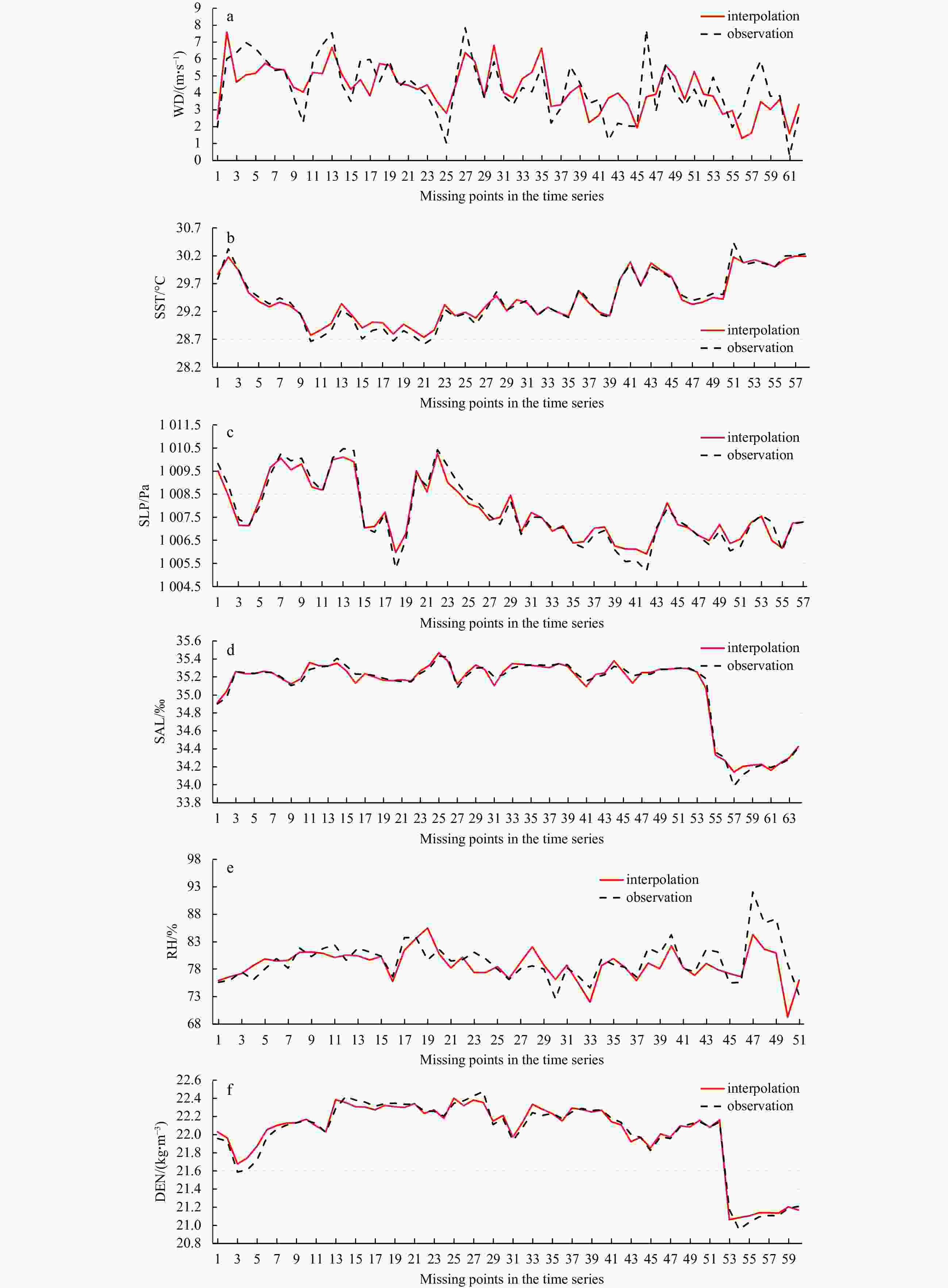
A1. Interpolation results with the data missing rate of 50%: WD (a), SST (b), SLP (c), SAL (d), RH (e), DEN (f).
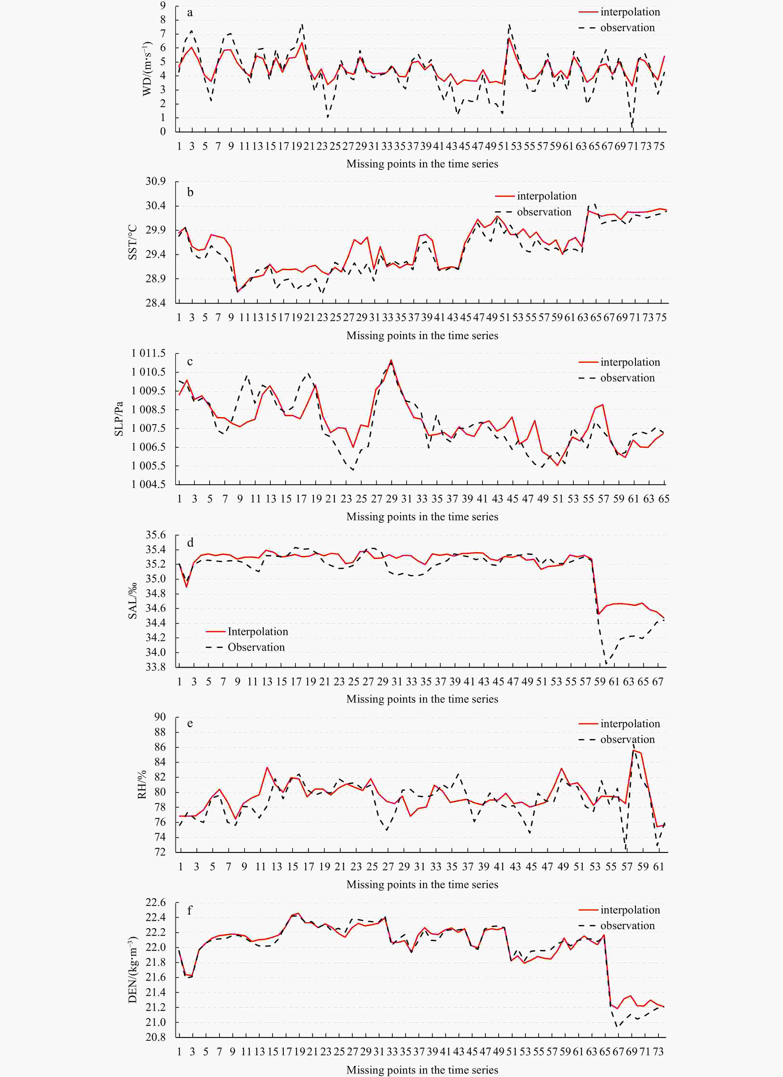
A2. Interpolation results with the data missing rate of 60%: WD (a), SST (b), SLP (c), SAL (d), RH (e), DEN (f).
Algorithm 1 GS algorithm Input $ V $ is variable set, $ D $ is complete data set of $ V $, $ {G}_{0} $ is an initial structure Output $ G $ is the optimal structure Step 1 Score the initial network structure ${G}_{0}\!\to\! oldscore$; Step 2 Perform arc addition, arc reduction and determine arc direction by IF, score the new network structure $ {G}'\!\to\! tempscore $; if $ tempscore\!>\!oldscore $ $ newscore\!\equiv\! tempscore $ and keep the corresponding arc operation; else $ newscore\!\equiv \!oldscore $ and discard the corresponding arc operation; end if Step 3 If $ newsore\!\to\! max $ return $ G\equiv {G}\!\to '\! $  下载: 导出CSV
Table 1. Discretization standard of ocean variables
Ocean variable WD SST SLP SAL RH DEN Interval 1 m/s 0.1°C 1 Pa 0.1‰ 1% 0.1 kg/m3 State label 1–10 1–26 1–9 1–17 1–24 1–19
下载: 导出CSV
Table 2. Discrete training time series
Variable Training data 1 d 2 d 3 d 4 d 5 d ··· 500 d 600 d WD/(m·s–1) 3 2 3 3 5 ··· 2 5 SST/°C 25 24 24 22 24 ··· 19 18 SLP/Pa 2 3 2 3 3 ··· 6 7 SAL/‰ 15 15 15 10 8 ··· 15 15 RH/% 8 12 14 17 10 ··· 9 7 DEN/(kg·m–3) 10 11 11 7 6 ··· 12 12
下载: 导出CSV
Table 3. Standardized IF matrix
Variable WD SST SLP SAL RH DEN WD \ 0.133 6 –0.002 5 –0.012 6 0.023 8 0.087 0 SST –0.000 3 \ 0.005 2 0.194 7 0.109 9 0.239 1 SLP 0.011 9 –0.011 8 \ 0.027 2 0.006 0 –0.023 9 SAL 0.003 0 0.119 3 0.037 1 \ 0.017 1 0.088 6 RH 0.039 4 0.096 2 0.006 7 –0.020 2 \ –0.018 6 DEN –0.005 2 0.259 3 0.028 1 0.347 4 0.066 9 \ Note: \ means it cannot be calculated.
下载: 导出CSV
Table 4. Conditional probability distribution of node
$ {\rm{SST}} $ Condition $P \left(\mathrm{S}\mathrm{S}\mathrm{T}\right|\mathrm{W}\mathrm{D})$ $ \mathrm{W}\mathrm{D}\!=\!1 $ $ \mathrm{W}\mathrm{D}\!=\!2 $ $ \mathrm{W}\mathrm{D}\!=\!3 $ $ \mathrm{W}\mathrm{D}\!=\!4 $ $ \mathrm{W}\mathrm{D}\!=\!5 $ $ \mathrm{W}\mathrm{D}\!=\!6 $ $ \mathrm{W}\mathrm{D}\!=\!7 $ $ \mathrm{W}\mathrm{D}\!=\!8 $ $ \mathrm{W}\mathrm{D}\!=\!9 $ $ \mathrm{W}\mathrm{D}\!=\!10 $ $ \mathrm{S}\mathrm{S}\mathrm{T}\!=\!1 $ 0 0 0 0 0 0 0.032 3 0 0 0 $ \mathrm{S}\mathrm{S}\mathrm{T}\!=\!2 $ 0 0 0 0 0 0.029 0 0.064 5 0.076 9 0 0 $ \mathrm{S}\mathrm{S}\mathrm{T}\!=\!3 $ 0 0 0 0 0.014 3 0.014 5 0 0 0 0 $ \mathrm{S}\mathrm{S}\mathrm{T}\!=\!4 $ 0 0 0 0 0.028 6 0.058 0 0.032 3 0 0 0 $ \mathrm{S}\mathrm{S}\mathrm{T}\!=\!5 $ 0 0 0 0.012 2 0.014 3 0.014 5 0.032 3 0 0 0 $ \mathrm{S}\mathrm{S}\mathrm{T}\!=\!6 $ 0 0 0.021 3 0.024 4 0.028 6 0.029 0 0.032 3 0.153 8 0 0 $ \mathrm{S}\mathrm{S}\mathrm{T}\!=\!7 $ 0 0.062 5 0 0.048 8 0.042 9 0.058 0 0.096 8 0.076 9 0 0 $ \mathrm{S}\mathrm{S}\mathrm{T}\!=\!8$ 0 0.031 3 0.021 3 0.012 2 0.042 9 0.043 5 0.032 3 0.076 9 0 0 $ \mathrm{S}\mathrm{S}\mathrm{T}\!=\!9 $ 0 0.031 3 0.042 6 0.109 8 0.014 3 0.014 5 0 0.153 8 0 0 $ \mathrm{S}\mathrm{S}\mathrm{T}\!=\!10$ 0.1 0.031 3 0.042 6 0.024 4 0.028 6 0.014 5 0 0.076 9 0 0 $ \mathrm{S}\mathrm{S}\mathrm{T}\!=\!11 $ 0 0.031 3 0.021 3 0.012 2 0.028 6 0.072 5 0.032 3 0 0 0 $ \mathrm{S}\mathrm{S}\mathrm{T}\!=\!12 $ 0 0 0.063 8 0.048 8 0.071 4 0.087 0 0 0.076 9 0 0 $ \mathrm{S}\mathrm{S}\mathrm{T}\!=\!13 $ 0.1 0 0.085 1 0.048 8 0.028 6 0.043 5 0.032 3 0 0 0 $ \mathrm{S}\mathrm{S}\mathrm{T}\!=\!14 $ 0.1 0 0 0.036 6 0.057 1 0.058 0 0.096 8 0.076 9 0 0 $ \mathrm{S}\mathrm{S}\mathrm{T}\!=\!15 $ 0 0.031 3 0.063 8 0.048 8 0.057 1 0.014 5 0.064 5 0.076 9 0.333 3 0 $ \mathrm{S}\mathrm{S}\mathrm{T}\!=\!16 $ 0 0.031 3 0.042 6 0.048 8 0.014 3 0.014 5 0.064 5 0 0 0 $ \mathrm{S}\mathrm{S}\mathrm{T}\!=\!17$ 0 0 0.042 6 0.012 2 0.028 6 0.043 5 0 0 0 0 $ \mathrm{S}\mathrm{S}\mathrm{T}\!=\!18 $ 0.2 0.031 3 0.085 1 0.073 2 0.114 3 0.014 5 0.064 0 0 0.333 3 0 $ \mathrm{S}\mathrm{S}\mathrm{T}\!=\!19 $ 0.1 0.156 3 0.021 3 0.122 0 0.128 6 0.072 5 0 0.076 9 0 0 $ \mathrm{S}\mathrm{S}\mathrm{T}\!=\!20 $ 0 0.062 5 0.063 8 0.085 4 0.014 3 0.058 0 0.096 8 0 0 0 $ \mathrm{S}\mathrm{S}\mathrm{T}\!=\!21 $ 0.2 0.187 5 0.148 9 0.134 1 0.071 4 0.058 0 0.032 3 0.076 9 0 1 $ \mathrm{S}\mathrm{S}\mathrm{T}\!=\!22$ 0 0.031 3 0.042 6 0.036 6 0.028 6 0.058 0 0.064 5 0 0 0 $ \mathrm{S}\mathrm{S}\mathrm{T}\!=\!23 $ 0.1 0.125 0 0.063 8 0.012 2 0.028 6 0.072 5 0.032 3 0 0 0 $ \mathrm{S}\mathrm{S}\mathrm{T}\!=\!24 $ 0 0.093 8 0.021 3 0.048 8 0.085 7 0.029 0 0.096 8 0 0.333 3 0 $ \mathrm{S}\mathrm{S}\mathrm{T}\!=\!25 $ 0.1 0.031 3 0.085 1 0 0.028 6 0.029 0 0 0 0 0 $ \mathrm{S}\mathrm{S}\mathrm{T}\!=\!26 $ 0 0.031 3 0.021 3 0 0 0 0 0 0 0 Note: WD=1, 2, ···, 10, and SST=1, 2, ···, 26 indicate WD and SST take different discrete states.
下载: 导出CSV
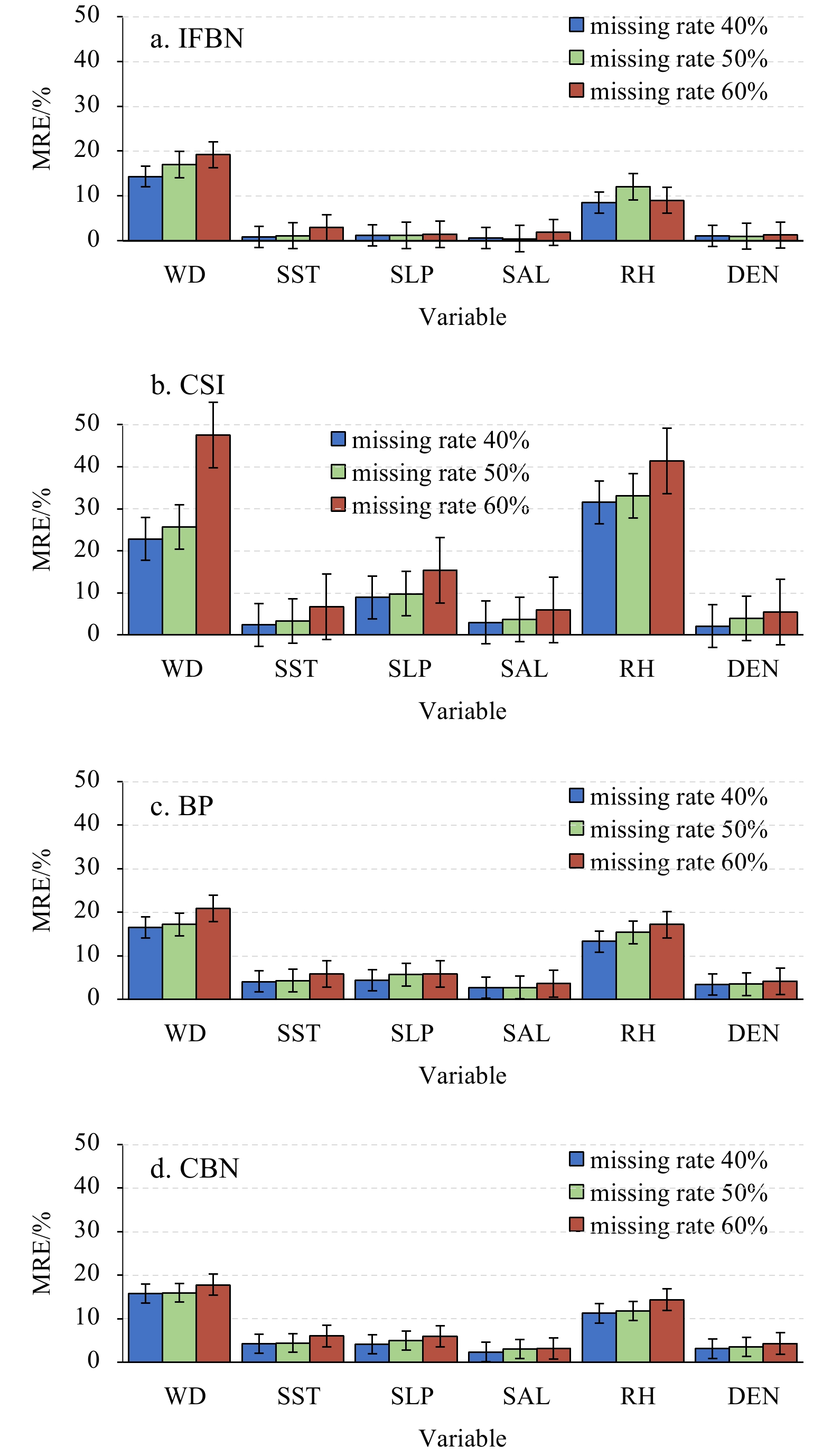
Table 5. TIC of each model under different missing rate
Missing rate Interpolation model WD SST SLP SAL RH DEN 40% IFBN 0.091 5 0.001 1 0.001 4 0.000 9 0.011 5 0.001 7 CSI 0.182 9 0.005 3 0.002 7 0.002 2 0.022 1 0.004 3 BP 0.095 6 0.003 3 0.002 5 0.001 6 0.014 1 0.003 5 CBN 0.089 7 0.003 6 0.002 2 0.001 8 0.013 9 0.003 3 50% IFBN 0.117 1 0.001 4 0.001 5 0.001 1 0.017 5 0.001 3 CSI 0.177 6 0.013 2 0.006 1 0.005 6 0.039 5 0.009 8 BP 0.119 4 0.005 8 0.004 3 0.003 4 0.025 2 0.014 3 CBN 0.112 1 0.005 6 0.004 5 0.003 7 0.031 1 0.012 7 60% IFBN 0.106 5 0.003 7 0.002 4 0.002 2 0.018 9 0.001 8 CSI 0.215 8 0.015 4 0.010 9 0.009 3 0.062 9 0.013 1 BP 0.138 2 0.008 3 0.007 4 0.006 5 0.040 7 0.012 1 CBN 0.141 2 0.007 9 0.007 5 0.006 1 0.039 6 0.011 9 Note: The bold numbers are the results obtained by proposed model.
下载: 导出CSV
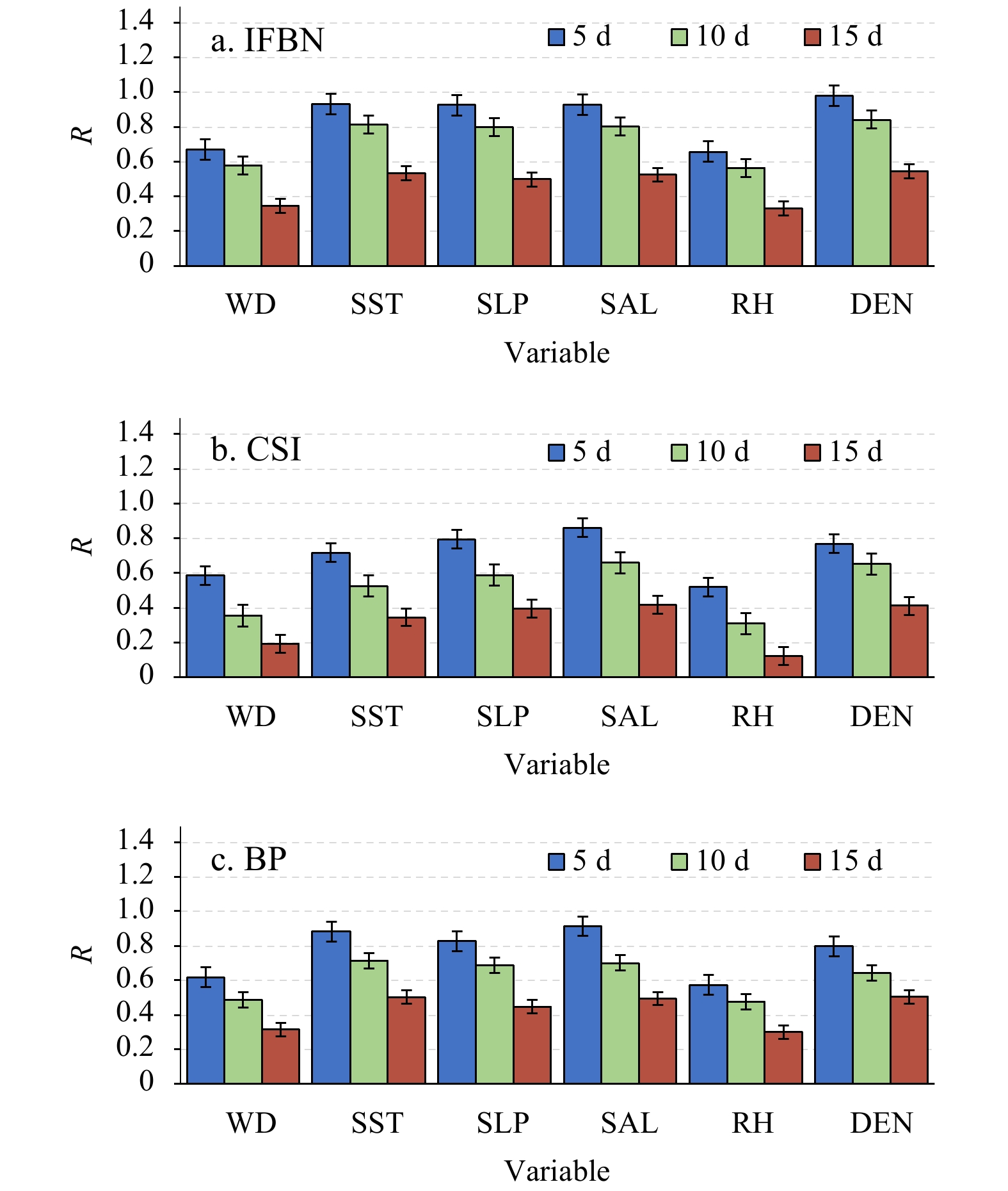
Table 6. R of each model under different missing rate
Missing rate Interpolation model WD SST SLP SAL RH DEN 40% IFBN 0.811 5 0.989 5 0.987 2 0.987 1 0.788 1 0.992 7 CSI 0.731 5 0.926 9 0.941 2 0.975 9 0.719 9 0.968 1 BP 0.636 6 0.915 7 0.935 3 0.985 9 0.720 5 0.973 6 CBN 0.701 1 0.914 8 0.939 8 0.984 6 0.731 6 0.975 4 50% IFBN 0.678 6 0.988 8 0.972 3 0.993 5 0.690 8 0.990 4 CSI 0.651 0 0.807 2 0.838 1 0.867 0 0.578 4 0.839 9 BP 0.512 7 0.943 8 0.905 7 0.975 5 0.596 1 0.816 5 CBN 0.611 4 0.915 2 0.902 1 0.969 8 0.601 3 0.824 1 60% IFBN 0.667 8 0.934 2 0.923 1 0.929 1 0.654 7 0.982 7 CSI 0.585 9 0.716 4 0.793 6 0.860 2 0.517 0 0.768 0 BP 0.618 3 0.883 2 0.826 5 0.973 8 0.574 4 0.798 3 CBN 0.609 7 0.892 1 0.799 8 0.976 1 0.584 2 0.801 1 Note: The bold numbers are the results obtained by proposed model.
下载: 导出CSV
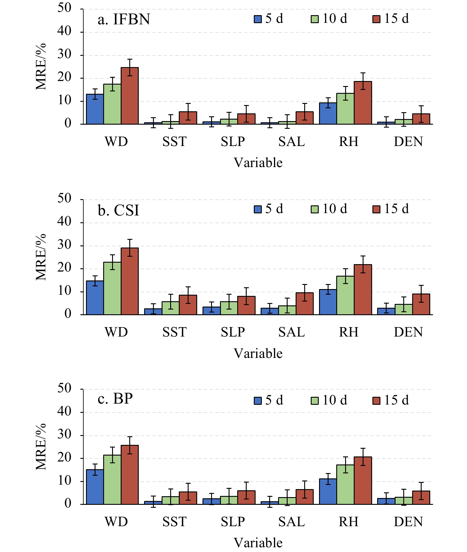
Table 7. The Maximum and averaged length of the consecutive missing data for each variable at different missing rate
Missing rate Statistics length WD SST SLP SAL RH DEN 40% maximum/d 4.00 5.00 4.00 4.00 4.00 3.00 average/d 1.59 1.92 1.78 1.78 1.48 1.32 50% maximum/d 6.00 5.00 7.00 7.00 6.00 7.00 average/d 2.32 2.46 3.56 3.91 3.64 2.98 60% maximum/d 8.00 8.00 7.00 9.00 8.00 9.00 average/d 3.78 5.23 4.16 5.35 4.62 5.01
下载: 导出CSV
Table 8. The imformation of new experiment data
Position name Peried Latitude-longitude coordinate A Jan. 1, 2013 to Jun. 30, 2015 5°N, 110°W B Apr. 1, 2009 to Jul. 31, 2012 12°N, 70°W C May 1, 2010 to Jan. 31, 2013 15°S, 90°E
下载: 导出CSV
Table 9. Comparative analysis of interpolation results with different model in Position A
Evaluation indicator Interpolation model WD SST SLP SAL RH DEN MRE IFBN 0.167 7 0.036 5 0.037 9 0.027 1 0.134 4 0.028 7 CSI 0.245 8 0.065 4 0.093 9 0.042 3 0.229 1 0.062 1 BP 0.191 5 0.056 4 0.041 2 0.035 9 0.179 9 0.038 1 TIC IFBN 0.140 9 0.002 6 0.002 2 0.000 5 0.023 9 0.002 7 CSI 0.179 4 0.005 8 0.004 3 0.004 4 0.075 2 0.014 3 BP 0.147 6 0.003 2 0.003 1 0.002 6 0.049 5 0.009 8 R IFBN 0.618 6 0.968 8 0.960 2 0.950 8 0.633 3 0.910 3 CSI 0.582 7 0.923 8 0.835 7 0.865 5 0.514 4 0.736 5 BP 0.601 2 0.946 9 0.908 1 0.917 1 0.577 1 0.819 9 Note: The bold numbers are the results obtained by proposed model.
下载: 导出CSV
Table 10. Comparative analysis of interpolation results with different model in Position B
Evaluation indicator Interpolation model WD SST SLP SAL RH DEN MRE IFBN 0.169 8 0.031 8 0.040 0 0.025 5 0.134 9 0.027 2 CSI 0.241 1 0.064 8 0.096 4 0.043 2 0.225 5 0.059 1 BP 0.189 3 0.055 2 0.039 0 0.033 1 0.176 4 0.035 6 TIC IFBN 0.136 4 0.005 3 0.002 1 0.000 3 0.021 5 0.003 9 CSI 0.175 4 0.008 8 0.005 9 0.002 0 0.078 6 0.014 0 BP 0.150 8 0.003 1 0.002 9 0.002 7 0.047 0 0.008 3 R IFBN 0.620 5 0.968 7 0.956 4 0.952 8 0.636 4 0.913 6 CSI 0.580 9 0.923 3 0.835 7 0.869 4 0.511 8 0.737 4 BP 0.605 7 0.948 4 0.912 7 0.921 7 0.581 4 0.820 4 Note: The bold numbers are the results obtained by proposed model.
下载: 导出CSV
Table 11. Comparative analysis of interpolation results with different model in Position C
Evaluation indicator Interpolation model WD SST SLP SAL RH DEN MRE IFBN 0.171 9 0.039 3 0.036 0 0.022 9 0.130 5 0.031 7 CSI 0.243 7 0.069 7 0.094 2 0.039 6 0.233 7 0.061 4 BP 0.194 1 0.052 7 0.037 9 0.040 0 0.174 9 0.042 2 TIC IFBN 0.143 4 0.003 3 0.003 2 0.000 4 0.026 6 0.003 5 CSI 0.178 2 0.005 5 0.001 9 0.007 7 0.078 4 0.011 9 BP 0.148 3 0.003 7 0.004 6 0.003 1 0.053 2 0.006 3 R IFBN 0.614 4 0.967 2 0.962 1 0.955 8 0.629 1 0.906 7 CSI 0.578 2 0.920 4 0.838 2 0.861 3 0.513 4 0.740 2 BP 0.601 5 0.949 8 0.907 6 0.916 5 0.574 7 0.820 7 Note: The bold numbers are the results obtained by proposed model.
下载: 导出CSV
-
[1] Bai Chengzu, Hong Mei, Wang Dong, et al. 2014. Evolving an information diffusion model using a genetic algorithm for monthly river discharge time series interpolation and forecasting. Journal of Hydrometeorology, 15(6): 2236–2249. doi: 10.1175/JHM-D-13-0184.1 [2] Barth A, Alvera-Azcárate A, Licer M, et al. 2020. DINCAE 1.0: a convolutional neural network with error estimates to reconstruct sea surface temperature satellite observations. Geoscientific Model Development, 13(3): 1609–1622. doi: 10.5194/gmd-13-1609-2020 [3] Bouckaert R R. 1994. A stratified simulation scheme for inference in Bayesian belief networks. In: Proceedings of the Tenth International Conference on Uncertainty in Artificial Intelligence. Seattle, WA: Morgan Kaufmann Publishers Inc, 110–117 [4] Bu Fanyu, Chen Zhikui, Zhang Qingchen. 2014. Incomplete big data imputation algorithm based on deep learning. Microelectronics & Computer (in Chinese), 31(12): 173–176 [5] Chickering D M. 2003. Optimal structure identification with greedy search. The Journal of Machine Learning Research, 3(3): 507–554 [6] Chickering M, Geiger D, Heckerman D. 1995. Learning Bayesian networks: search methods and experimental results. In: Proceedings of Fifth Conference on Artificial Intelligence and Statistics. Lauderdale, FL: Society for Artificial Intelligence in Statistics [7] Cooper G F, Herskovits E. 1992. A Bayesian method for the induction of probabilistic networks from data. Machine Learning, 9(4): 309–347 [8] Gasca M, Sauer T. 2000. Polynomial interpolation in several variables. Advances in Computational Mathematics, 12(4): 377. doi: 10.1023/A:1018981505752 [9] Gong Yi, Dong Chen. 2010. Data patching method based on Bayesian network. Journal of Shenyang University of Technology (in Chinese), 32(1): 79–83 [10] Huang Rong, Hu Zeyong, Guan Ting, et al. 2014. Interpolation of temperature data in northern Qinghai-Xizang Plateau and preliminary analysis on its recent variation. Plateau Meteorology (in Chinese), 33(3): 637–646 [11] Jiang Dong, Fu Jingying, Huang Yaohuan, et al. 2011. Reconstruction of time series data of environmental parameters: methods and application. Journal of Geo-Information Science (in Chinese), 13(4): 439–446. doi: 10.3724/SP.J.1047.2011.00439 [12] Kaplan A, Kushnir Y, Cane M A. 2000. Reduced space optimal interpolation of historical marine sea level pressure: 1854−1992. Journal of Climate, 13(16): 2987–3002. doi: 10.1175/1520-0442(2000)013<2987:RSOIOH>2.0.CO;2 [13] Li H. 2006. Lost data filling algorithm based on EM and Bayesian network. Computer Engineering and Applications, 46(5): 123–125 [14] Li Ming, Hong Mei, Zhang Ren. 2018a. Improved Bayesian network-based risk model and its application in disaster risk assessment. International Journal of Disaster Risk Science, 9(2): 237–248. doi: 10.1007/s13753-018-0171-z [15] Li Haitao, Jin Guang, Zhou Jinglun, et al. 2008. Survey of Bayesian network inference algorithms. Systems Engineering and Electronics (in Chinese), 30(5): 935–939 [16] Li Ming, Liu Kefeng. 2018. Application of intelligent dynamic Bayesian network with wavelet analysis for probabilistic prediction of storm track intensity index. Atmosphere, 9(6): 224. doi: 10.3390/atmos9060224 [17] Li Ming, Liu Kefeng. 2019. Causality-based attribute weighting via information flow and genetic algorithm for naive Bayes classifier. IEEE Access, 7: 150630–150641. doi: 10.1109/ACCESS.2019.2947568 [18] Li Ming, Liu Kefeng. 2020. Probabilistic prediction of significant wave height using dynamic Bayesian network and information flow. Water, 12(8): 2075. doi: 10.3390/w12082075 [19] Li Ming, Zhang Ren, Hong Mei, et al. 2018b. Improved structure learning algorithm of Bayesian network based on information flow. Systems Engineering and Electronics (in Chinese), 40(6): 1385–1390 [20] Liang Xiangsan. 2008. Information flow within stochastic dynamical systems. Physical Review: E, Statistical, Nonlinear, and Soft Matter Physics, 78(3): 031113 [21] Liang Xiangsan. 2014. Unraveling the cause-effect relation between time series. Physical Review: E, Statistical, Nonlinear, and Soft Matter Physics, 90(5−1): 052150 [22] Liang Xiangsan. 2015. Normalizing the causality between time series. Physical Review: E, Statistical, Nonlinear, and Soft Matter Physics, 92(2): 022126. doi: 10.1103/PhysRevE.92.022126 [23] Liu Meiling, Liu Xiangnan, Liu Da, et al. 2015. Multivariable integration method for estimating sea surface salinity in coastal waters from in situ data and remotely sensed data using random forest algorithm. Computers & Geosciences, 75: 44–56 [24] Liu Dayou, Wang Fei, Lu Yinan, et al. 2001. Research on learning Bayesian network structure based on genetic algorithms. Journal of Computer Research & Development (in Chinese), 38(8): 916–922 [25] Liu Tian, Yang Kun, Qin Jun, et al. 2018. Construction and applications of time series of monthly precipitation at weather stations in the central and eastern Qinghai-Tibetan Plateau. Plateau Meteorology (in Chinese), 37(6): 1449–1457 [26] Liu Junna, Zhang Yousheng. 2006. An adaptive joint tree algorithm. In: System Simulation Technology and Its Application Academic Exchange Conference Proceedings. Hefei: China System Simulation Society [27] Pearl J. 1998. Probabilistic Reasoning in Intelligent Systems: Networks of Plausible Inference. Berlin: Elsevier Inc [28] Sheng Zheng, Shi Hanqing, Ding Youzhuan. 2009. Using DINEOF method to reconstruct missing satellite remote sensing sea temperature data. Advances in Marine Science (in Chinese), 27(2): 243–249 [29] Shi Zhifu. 2012. Bayesian Network Theory and its Application in Military System (in Chinese). Beijing: Defense Industry Press [30] Wang Tong, Yang Jie. 2010. A heuristic method for learning Bayesian networks using discrete particle swarm optimization. Knowledge and Information Systems, 24(2): 269–281. doi: 10.1007/s10115-009-0239-6 [31] Xu Zilong, Xing Zuoxia, Ma Shichang. 2018. Wind power data missing data processing based on adaptive BP neural network. In: Proceedings of the 15th Shenyang Scientific Academic Annual Meeting. Shenyang: Shenyang Science and Technology Association [32] Yao Zizhen. 2006. A Regression-based K nearest neighbor algorithm for gene function prediction from heterogeneous data. BMC Bioinformatics, 7(1): S11. doi: 10.1186/1471-2105-7-11 [33] Zhang Chan. 2013. A support vector machine-based missing values filling algorithm. Computer Applications and Software (in Chinese), 30(5): 226–228 [34] Zheng Chongwei, Chen Yunge, Zhan Chao, et al. 2019. Source tracing of the swell energy: A case study of the Pacific Ocean. IEEE Access, 7: 139264–139275. doi: 10.1109/ACCESS.2019.2943903 [35] Zheng Chongwei, Liang Bingchen, Chen Xuan, et al. 2020. Diffusion characteristics of swells in the North Indian Ocean. Journal of Ocean University of China, 19(3): 479–488. doi: 10.1007/s11802-020-4282-y [36] Zhou Zhihua. 2016. Machine Learning (in Chinese). Beijing: Tsinghua University Press [37] Zhu Ke. 2016. Bootstrapping the portmanteau tests in weak auto-regressive moving average models. Journal of the Royal Statistical Society: Series B, 78(2): 463–485. doi: 10.1111/rssb.12112 -


 点击查看大图

计量
- 文章访问数: 423
- HTML全文浏览量: 136
- PDF下载量: 14
- 被引次数: 0

