

-
Abstract: Based on a coupled ocean-sea ice model, this study investigates how changes in the mean state of the atmosphere in different CO2 emission scenarios (RCP 8.5, 6.0, 4.5 and 2.6) may affect the sea ice in the Bohai Sea, China, especially in the Liaodong Bay, the largest bay in the Bohai Sea. In the RCP 8.5 scenario, an abrupt change of the atmospheric state happens around 2070. Due to the abrupt change, wintertime sea ice of the Liaodong Bay can be divided into 3 periods: a mild decreasing period (2021–2060), in which the sea ice severity weakens at a near-constant rate; a rapid decreasing period (2061–2080), in which the sea ice severity drops dramatically; and a stabilized period (2081–2100). During 2021–2060, the dates of first ice are approximately unchanged, suggesting that the onset of sea ice is probably determined by a cold-air event and is not sensitive to the mean state of the atmosphere. The mean and maximum sea ice thickness in the Liaodong Bay is relatively stable before 2060, and then drops rapidly in the following decade. Different from the RCP 8.5 scenario, atmospheric state changes smoothly in the RCP 6.0, 4.5 and 2.6 scenarios. In the RCP 6.0 scenario, the sea ice severity in the Bohai Sea weakens with time to the end of the twenty-first century. In the RCP 4.5 scenario, the sea ice severity weakens with time until reaching a stable state around the 2070s. In the RCP 2.6 scenario, the sea ice severity weakens until the 2040s, stabilizes from then, and starts intensifying after the 2080s. The sea ice condition in the other bays of the Bohai Sea is also discussed under the four CO2 emissions scenarios. Among atmospheric factors, air temperature is the leading one for the decline of the sea ice extent. Specific humidity also plays an important role in the four scenarios. The surface downward shortwave/longwave radiation and meridional wind only matter in certain scenarios, while effects from the zonal wind and precipitation are negligible.
-
Key words:
- sea ice /
- Liaodong Bay /
- RCP scenarios /
- NEMO /
- LIM2
-
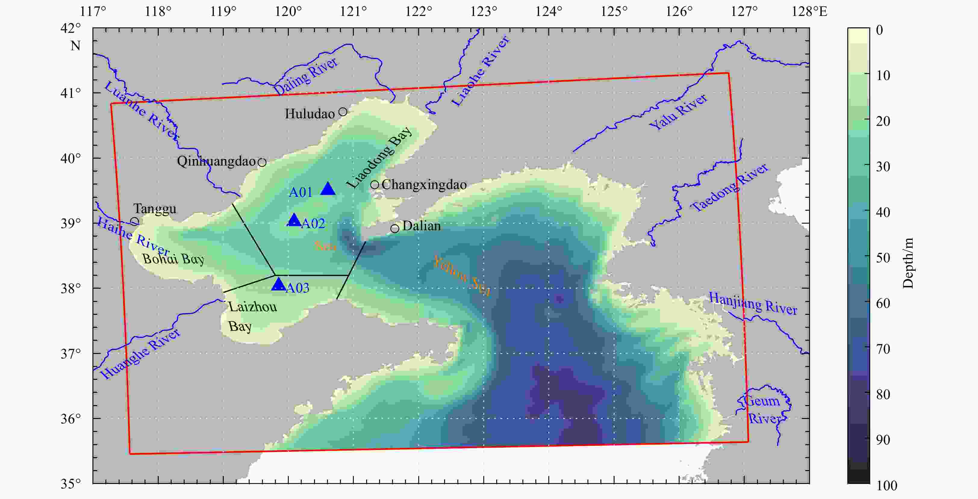
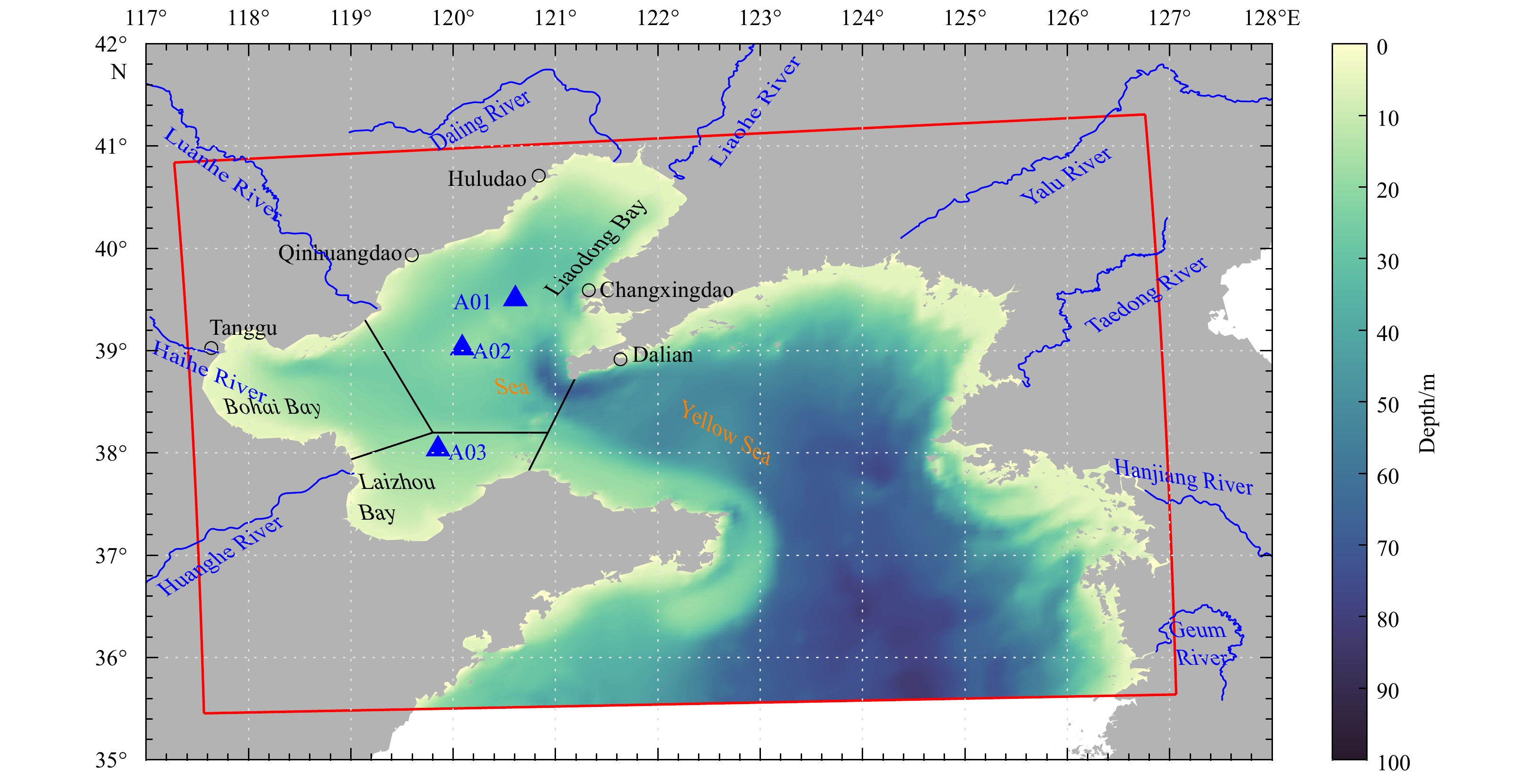
Figure 1. Topography in the model domain. The edge of the domain is marked by the red lines. The blue lines indicate major rivers in this region, and the blue triangles indicate locations of buoys where sea surface temperature is measured.
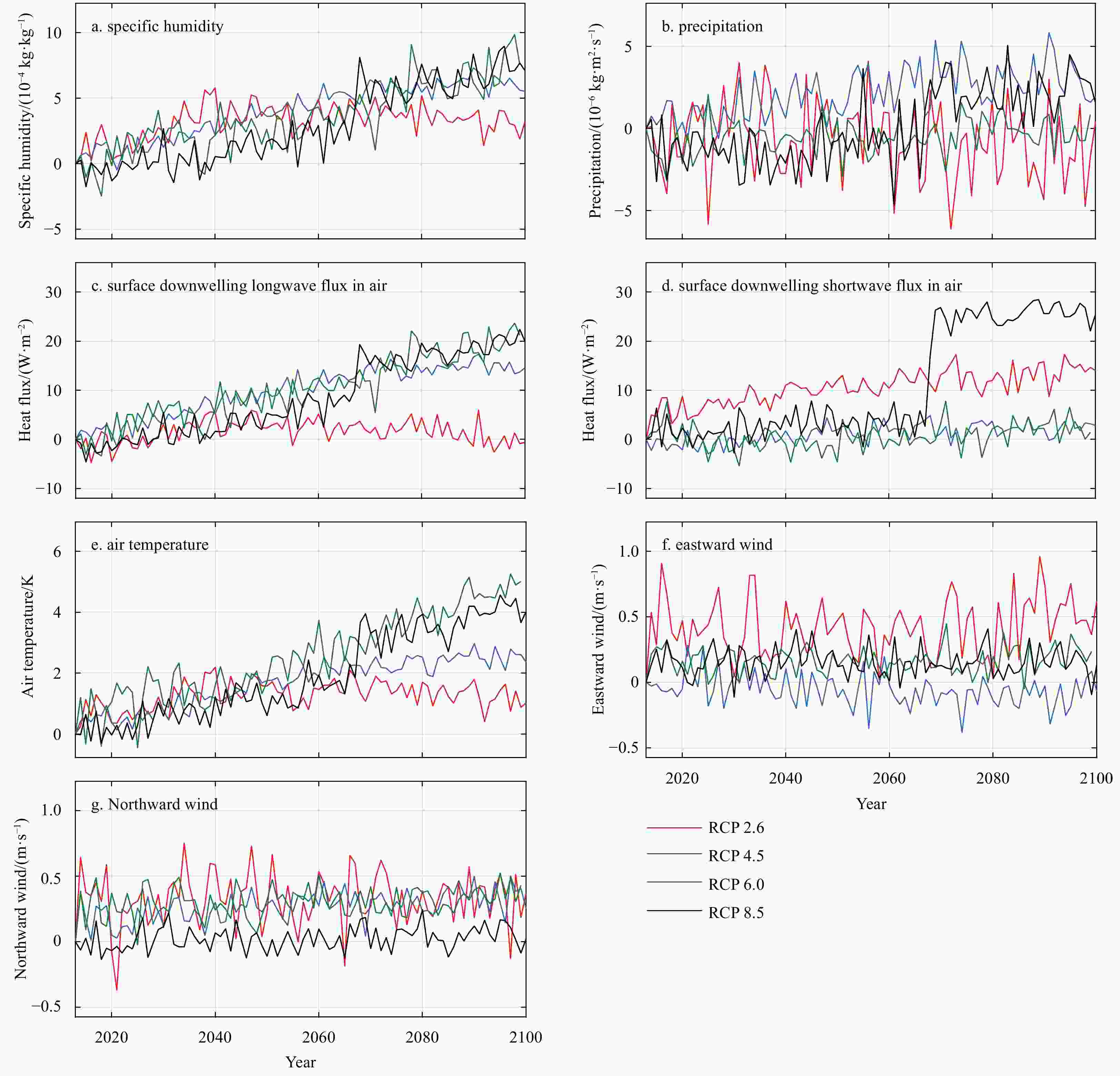
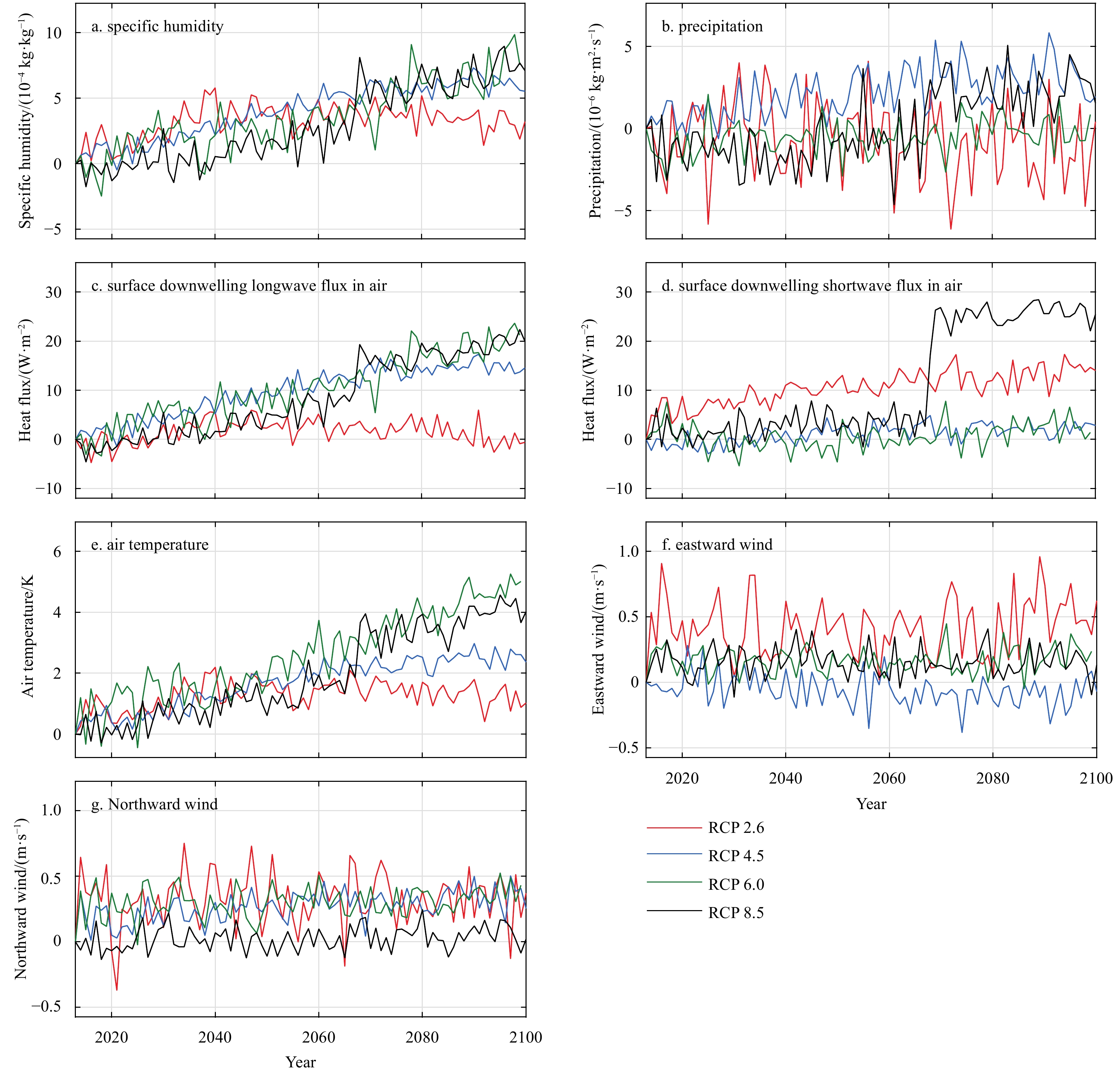
Figure 2. Changes of wintertime (November to March) averaged 2-m specific humidity (a), precipitation (b), surface downward longwave radiation (c), surface downward shortwave radiation (d), 2-m air temperature (e), and 10-m wind in the zonal (f) and meridional (g) directions above the Bohai Sea in different CO2 emission scenarios compared to the winter of 2012–2013.
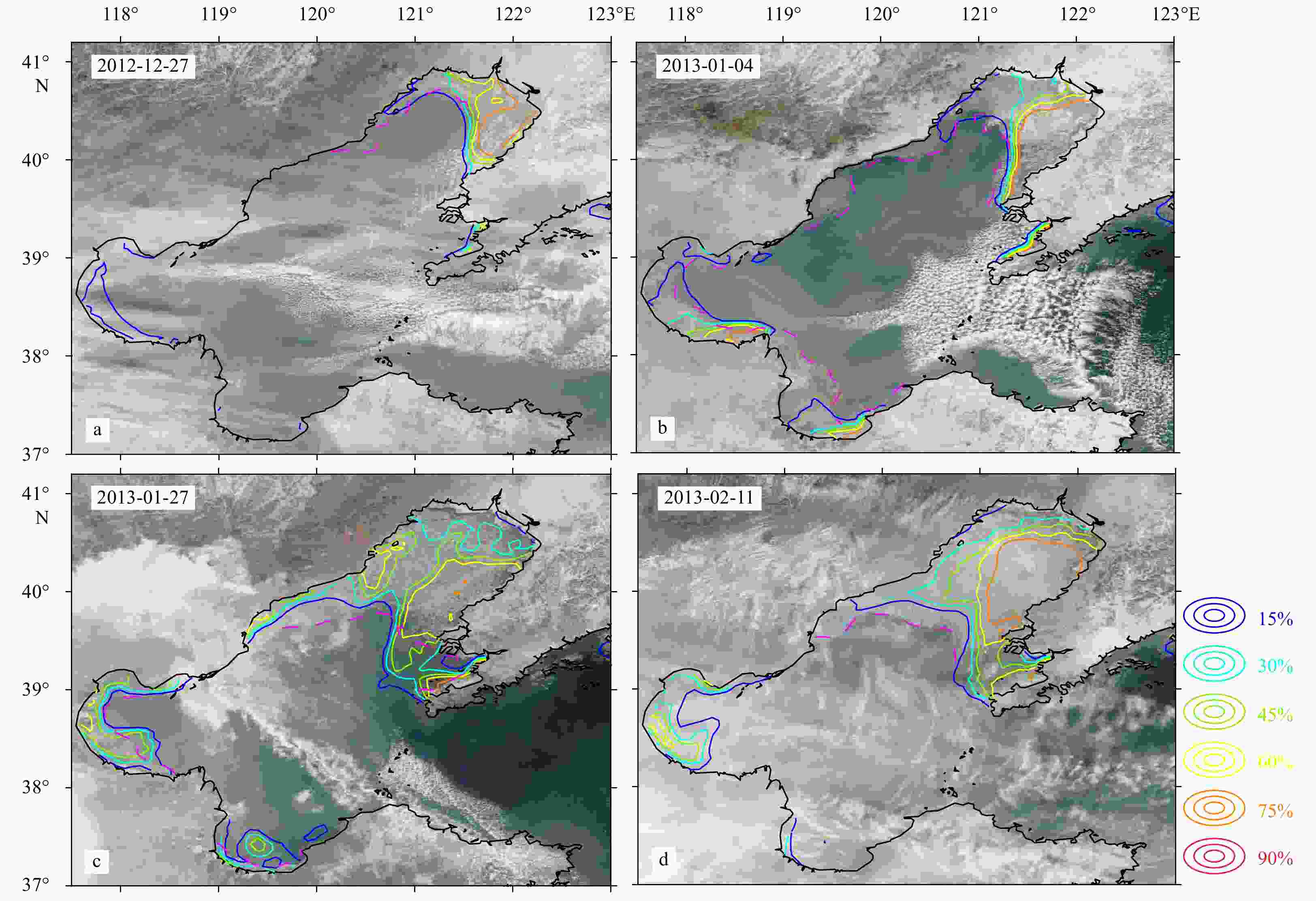
Figure 3. True color images from MODIS (background image) and contours of sea ice concentration (solid colorful lines) from the control experiment. The dashed lines indicate sea ice extent subjectively derived from the satellite images.
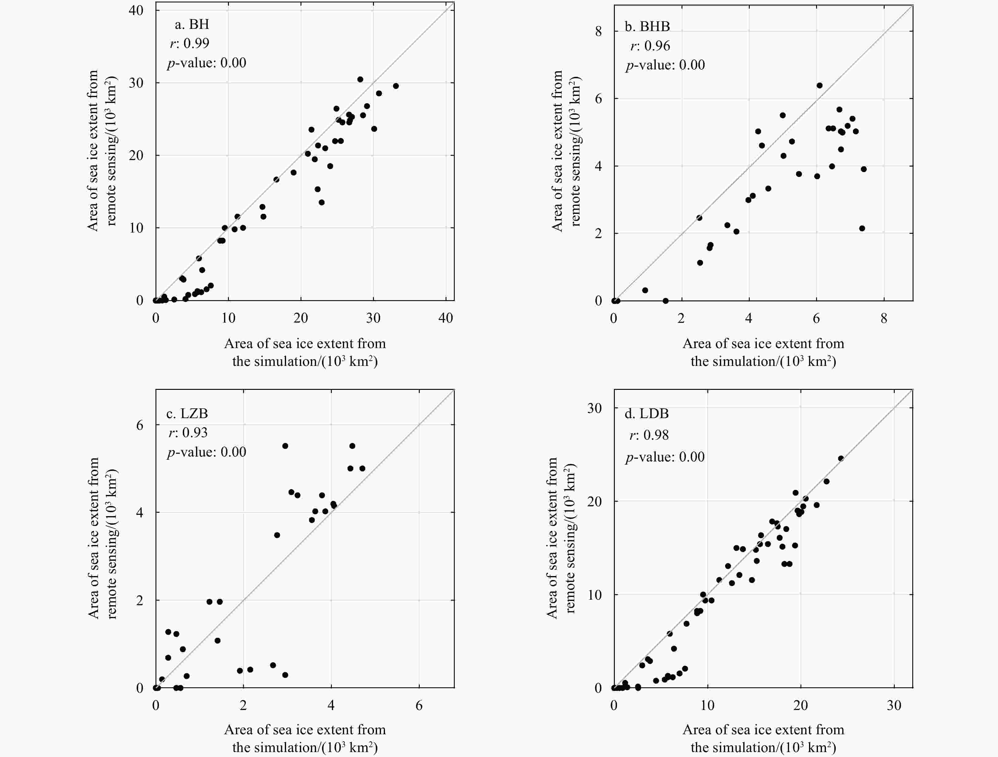
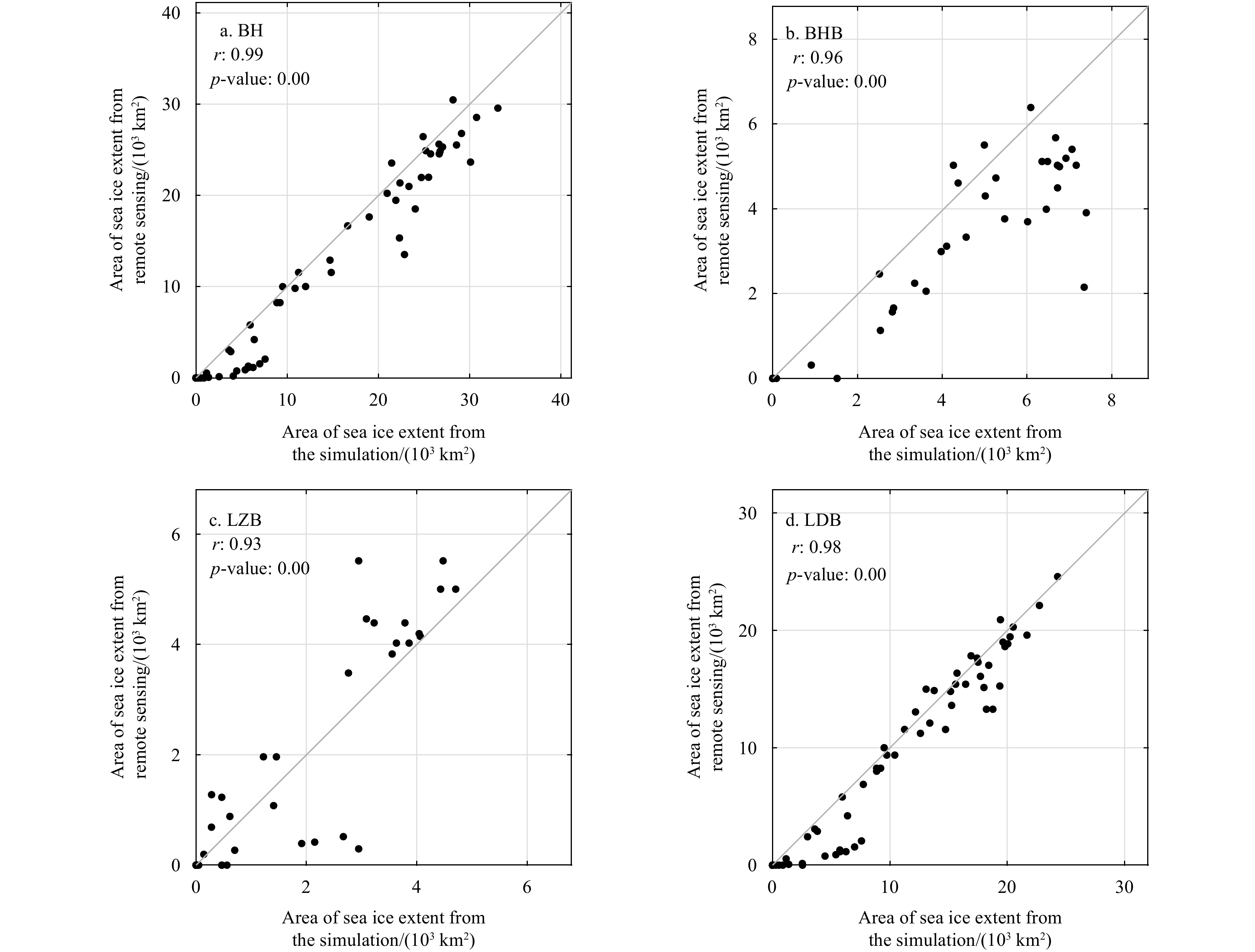
Figure 4. Area of sea surface occupied by sea ice with a concentration of more than 10% from the control run (x axis) and remote sensing (y axis) in the Bohai Sea (BH, a), the Bohai Bay (BHB, b), the Laizhou Bay (LZB, c) and the Liaodong Bay (LDB, d). The correlation coefficient (r) and corresponding p-value are indicated at the upper-left corner of each panel.
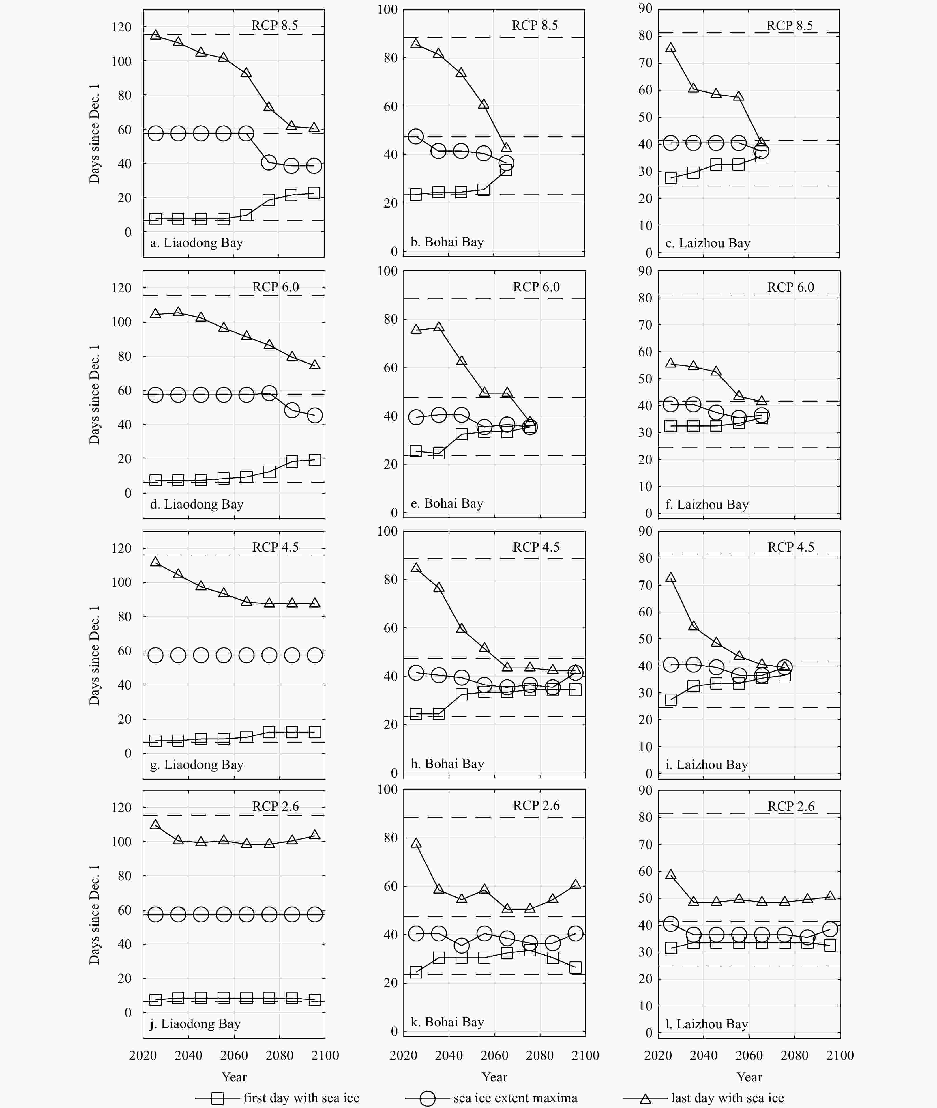
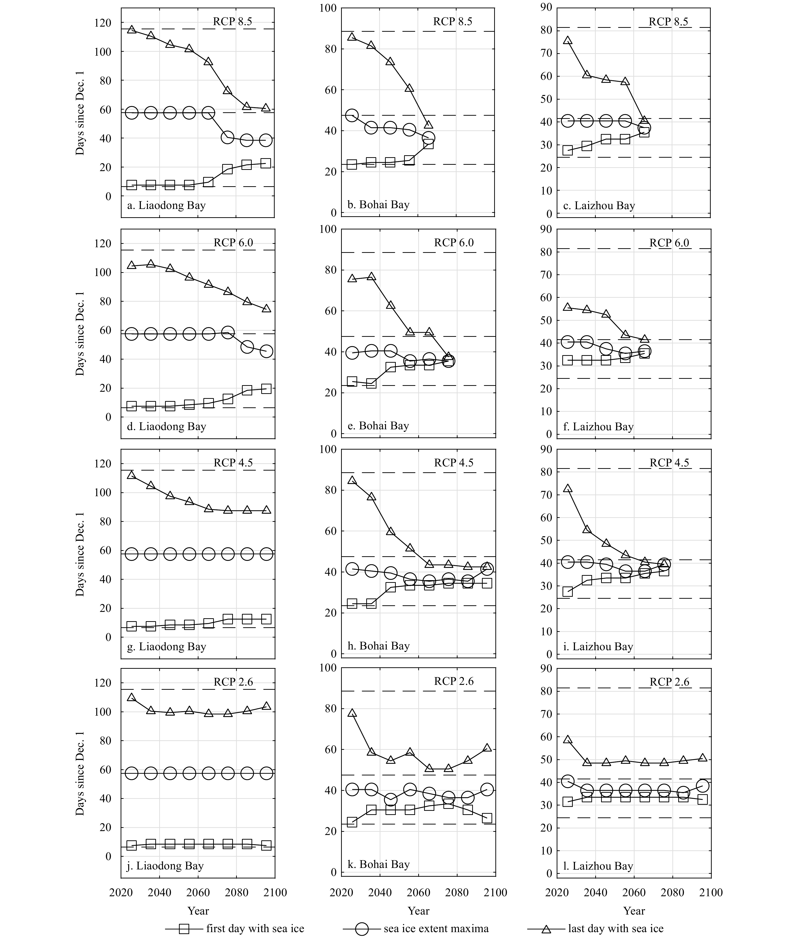
Figure 5. The date of first ice, maximum sea ice extent and last ice in different CO2 emission scenarios derived from sensitive experiments Exp-SE-a. The dashed horizontal lines indicate the corresponding values in the control experiment for the winter of 2012–2013.
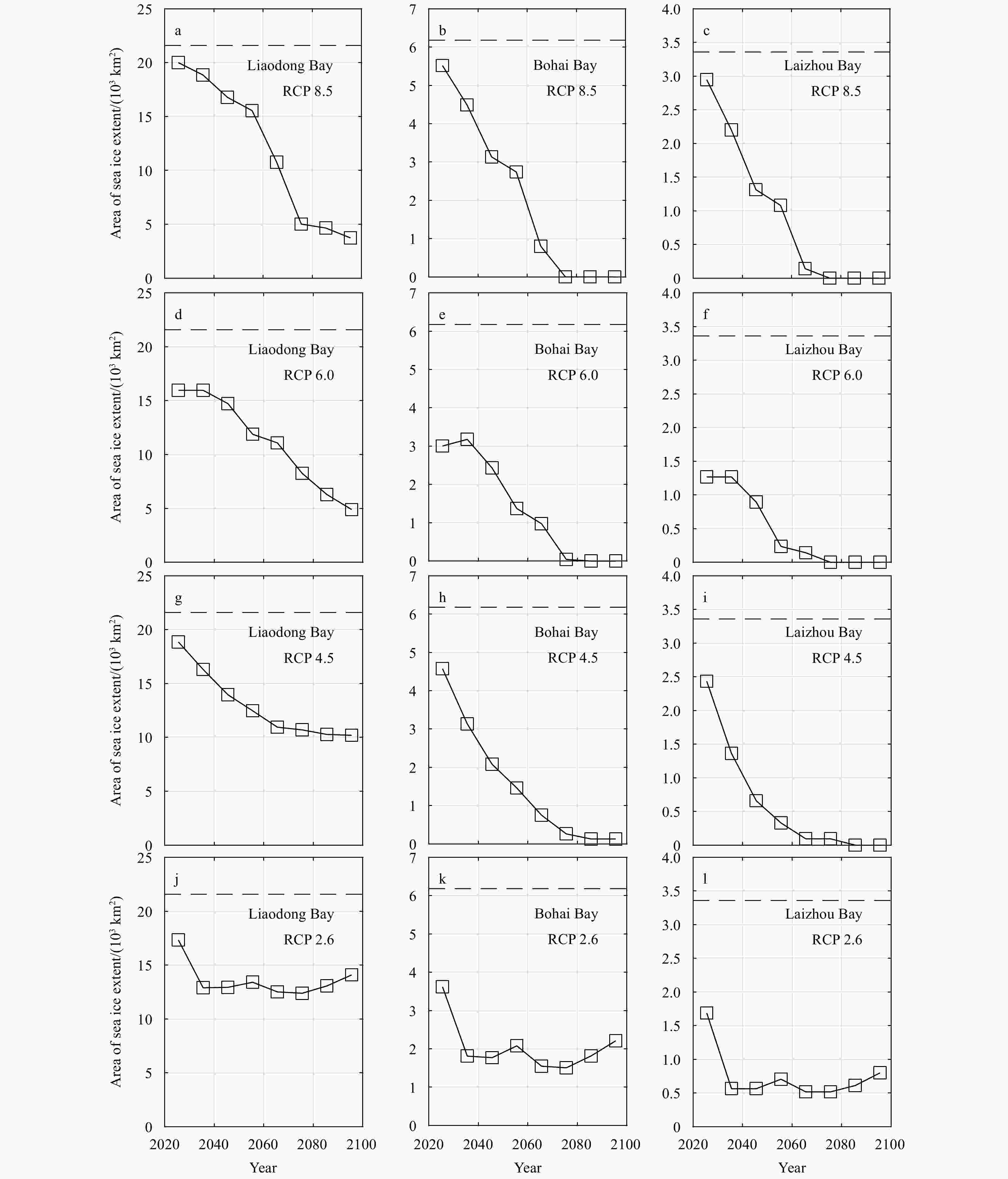
Figure 6. The area of max sea ice extent in different CO2 emission scenarios from sensitive experiments Exp-SE-a. The dashed horizontal lines indicate the corresponding values in the control experiment for the winter of 2012–2013.
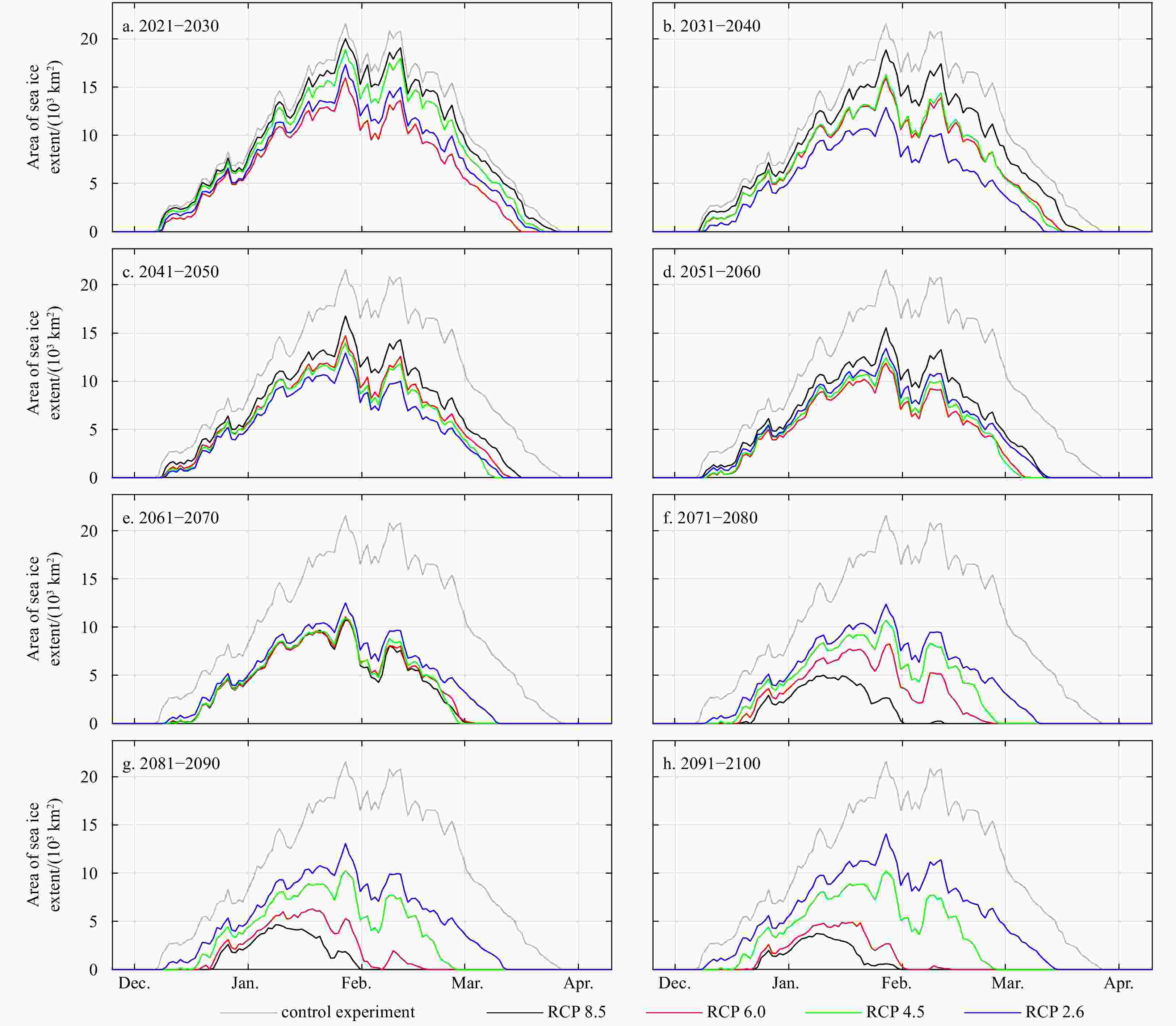
Figure 7. Area of sea ice extent with a concentration of more than 15% in the Liaodong Bay from the control experiment and the sensitive experiments Exp-SE-a.
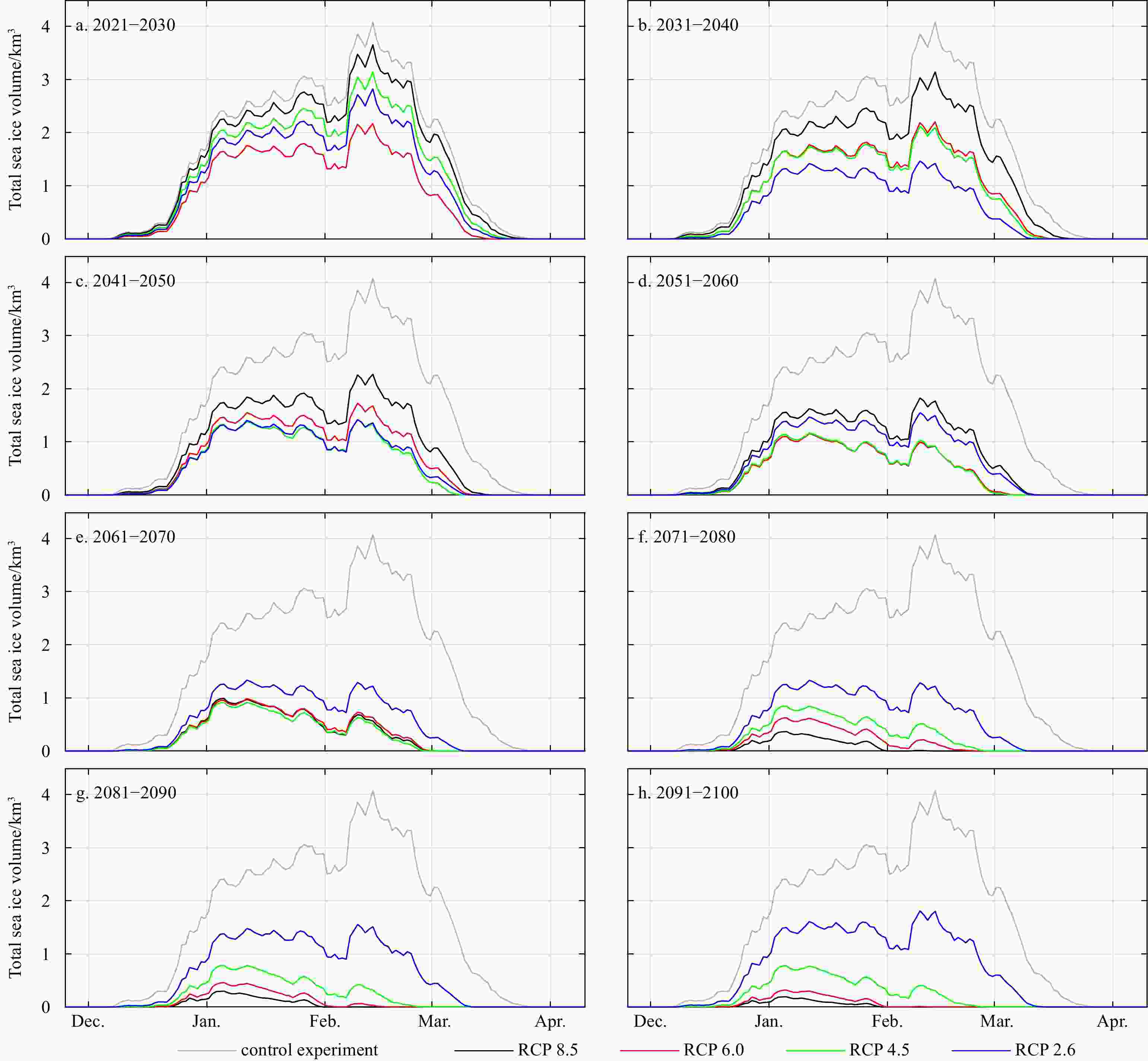
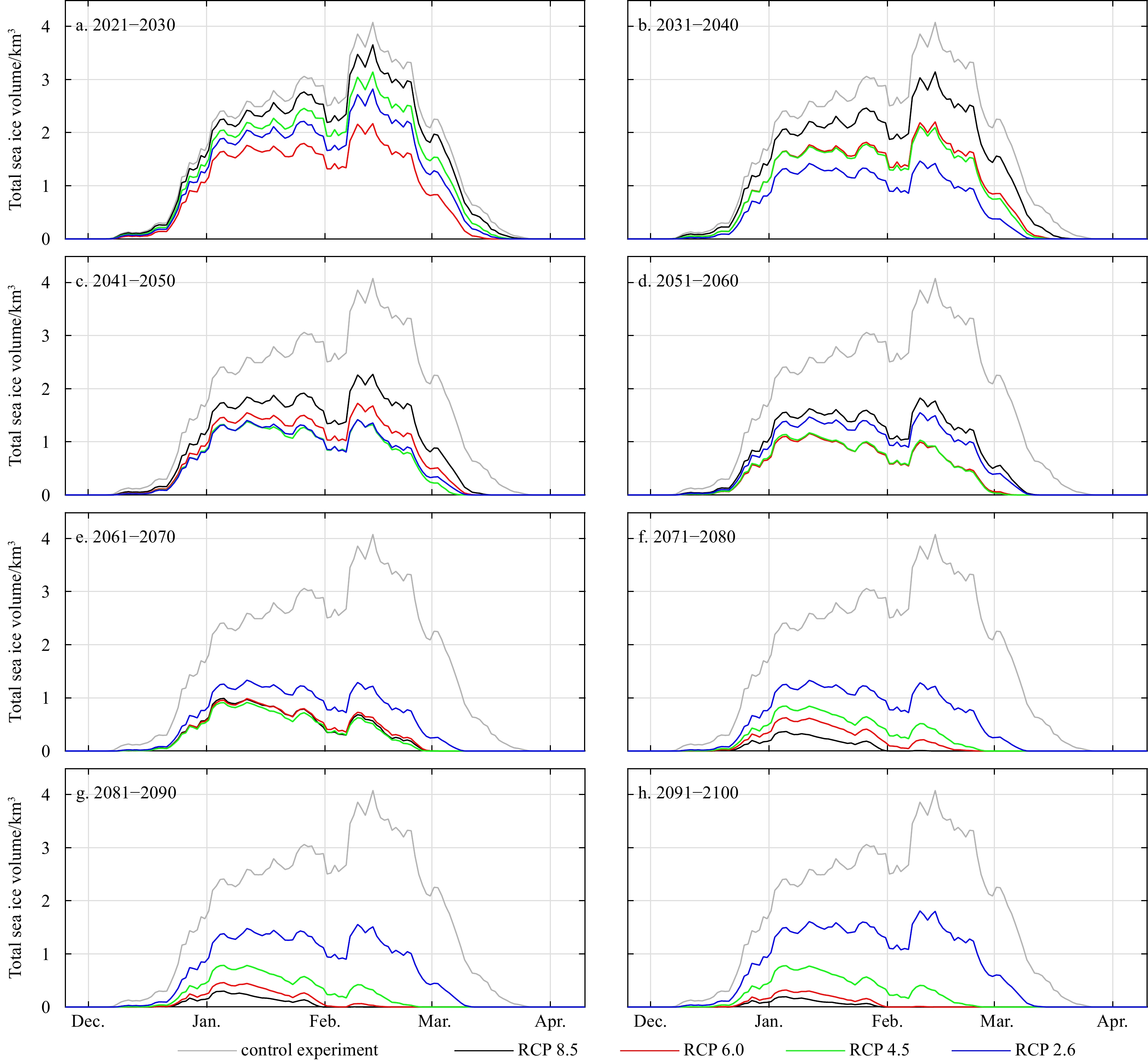
Figure 8. Total volume of sea ice in the Liaodong Bay from the control experiment and the sensitive experiments Exp-SE-a.
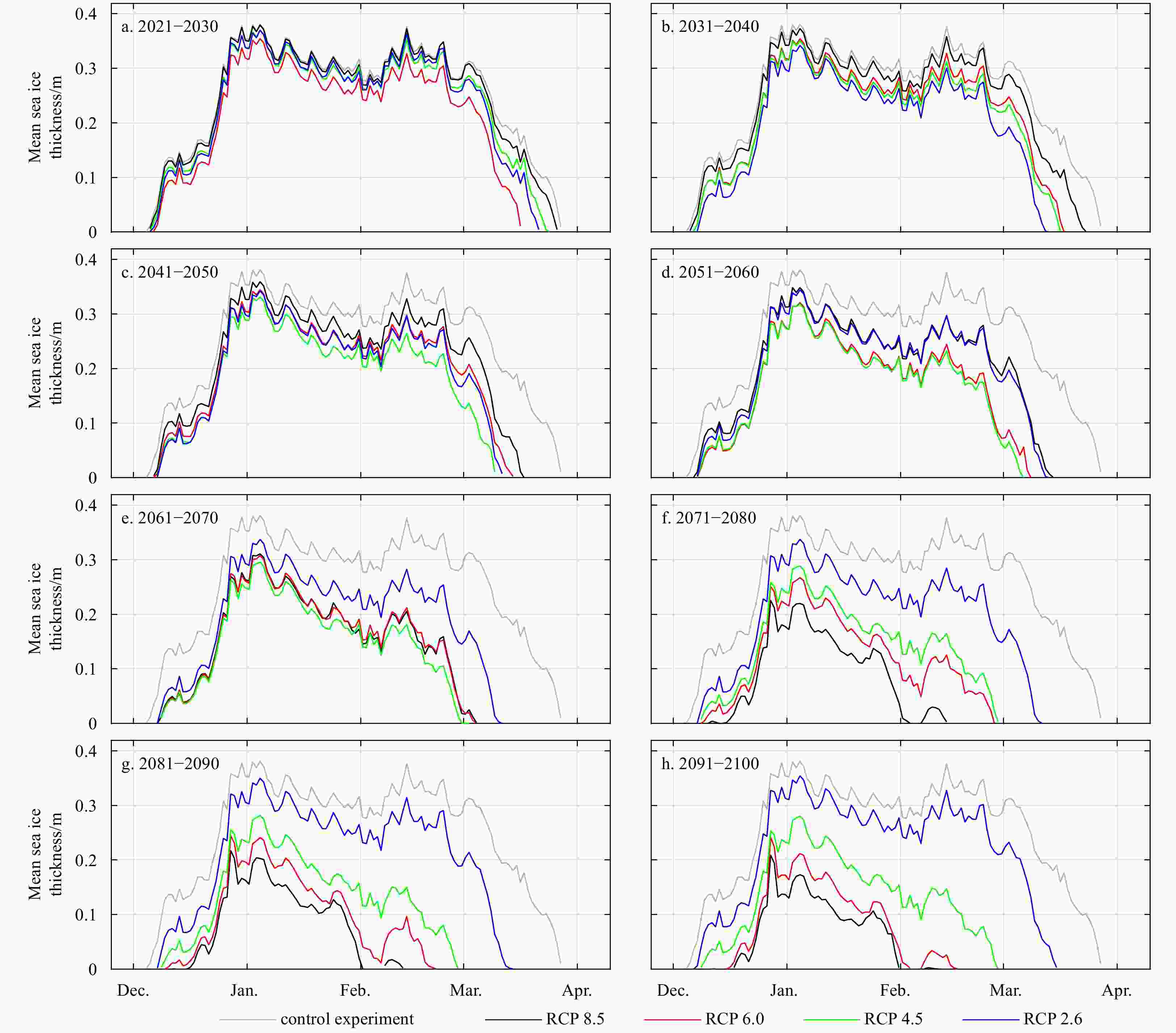
Figure 9. Mean thickness of the sea ice in the Liaodong Bay from the control experiment and the sensitive experiments Exp-SE-a.
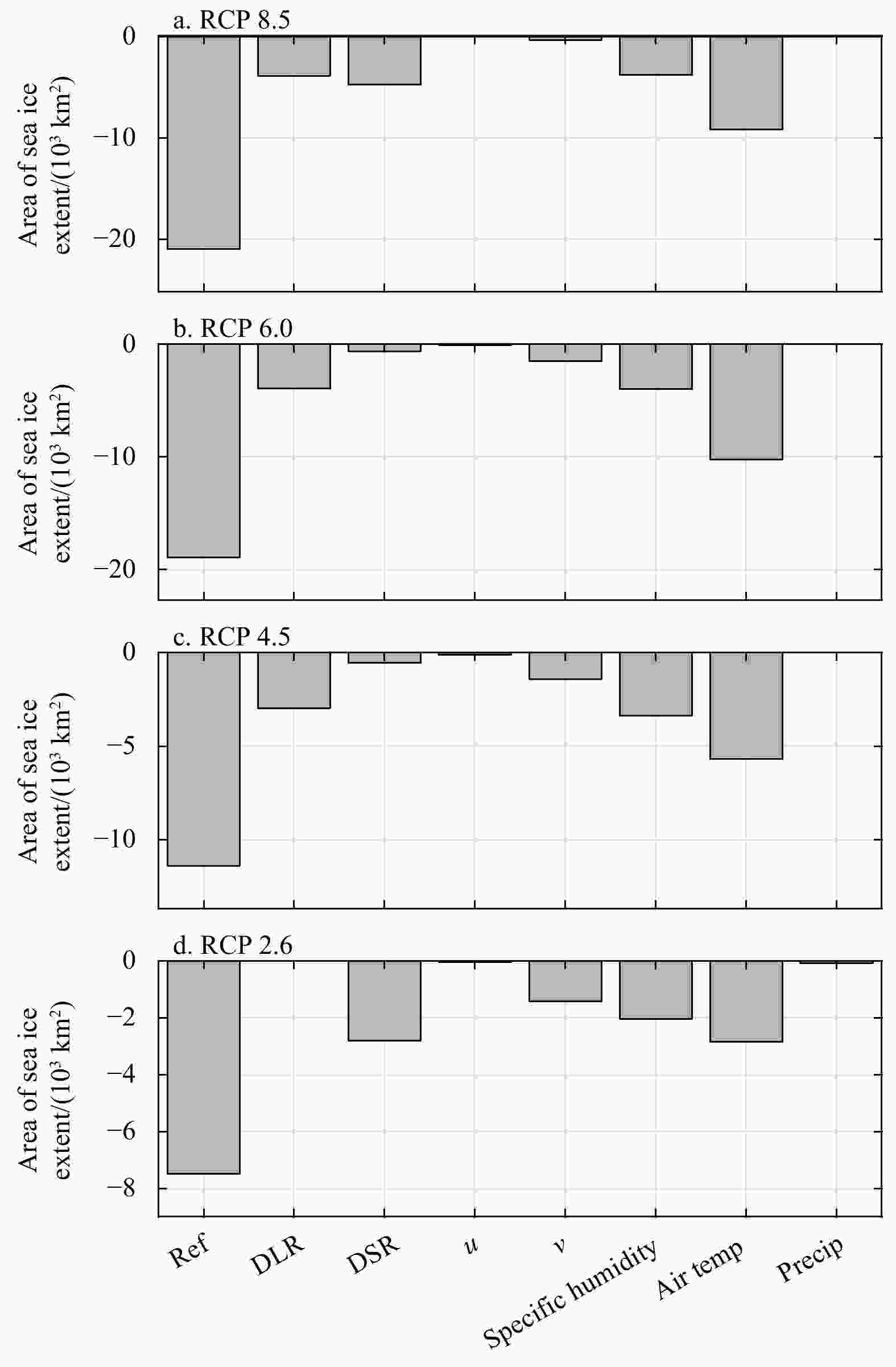
Figure 10. The role of each atmospheric factor in the sea ice extent decline to the end of the 21st century. The first bar of each panel (noted as Ref) shows the difference between sea ice extent area on January 27 in the winter of the 2090s (from the sensitive experiments Exp-SE-a) and the winter of 2012–2013 (from the control experiment) in the Liaodong Bay. The other bars indicate the area differences between the control experiment and the sensitive experiments Exp-SE-b, in which only one of the atmospheric variables (noted in x-axis) is edited according to the climate forecasts for the 2090s and the others remain unchanged from the control experiment.

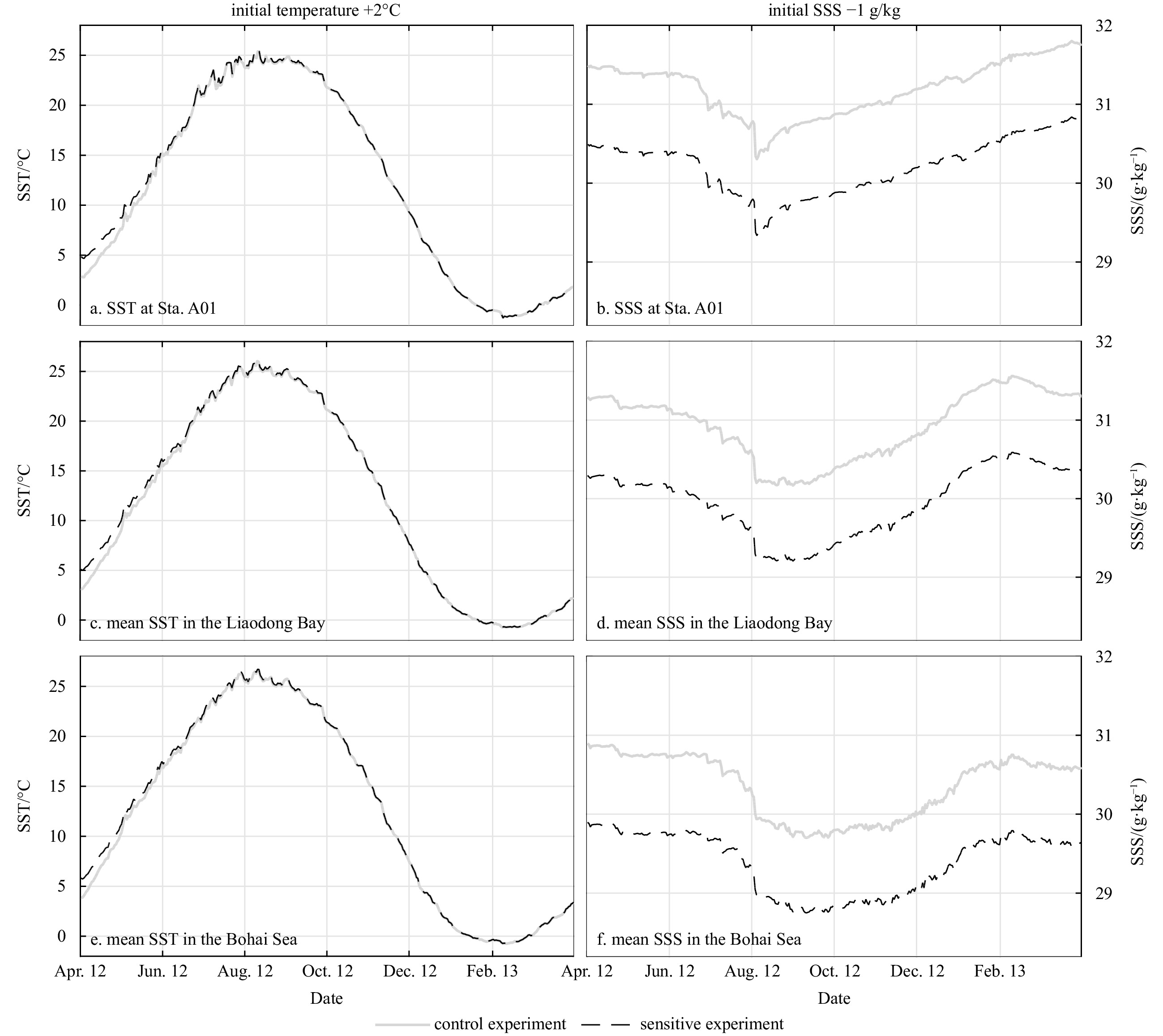
A1. Sea surface temperature (SST, a, c, e) from the control experiment (solid grey lines) and the sensitive experiment Exp-Ini-Temp (dashed black lines), whose initial temperature is 2°C higher than the control experiment; sea surface salinity (SSS, b, d, f) from the control experiment (solid grey lines) and the sensitive experiment Exp-Ini-Salt (dashed black lines), whose initial salinity is 1 g/kg lower than the control experiment. The location of station A01 is shown in Fig. 1.
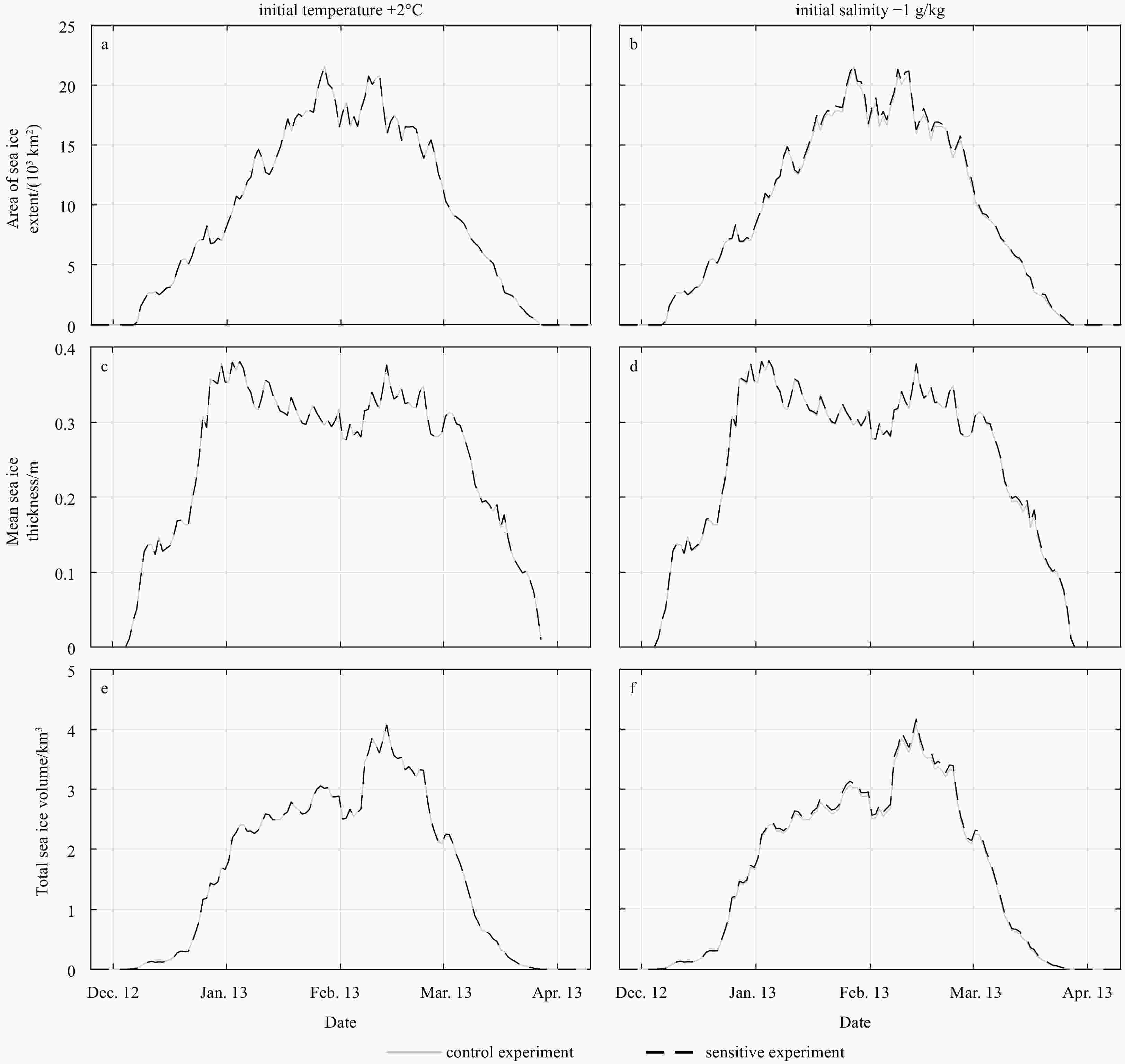
A2. Area of sea ice (a, b), Mean sea ice thickness (c, d), and total sea ice volume (e, f) from the control experiment (solid grey lines) and two sensitive experiments (dashed black lines), Exp-Ini-Temp (left panels), whose initial temperature is 2°C higher than the control experiment, and Exp-Ini-Salt (right panels), whose initial salinity is 1 g/kg lower than the control experiment.
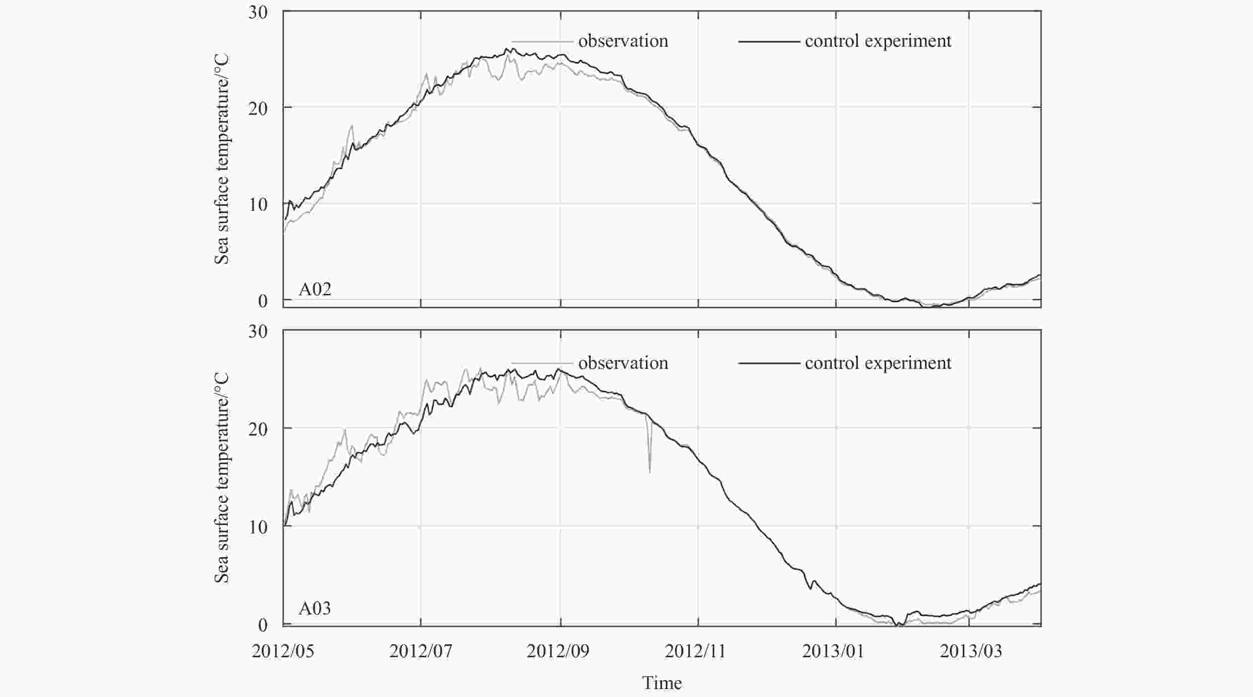
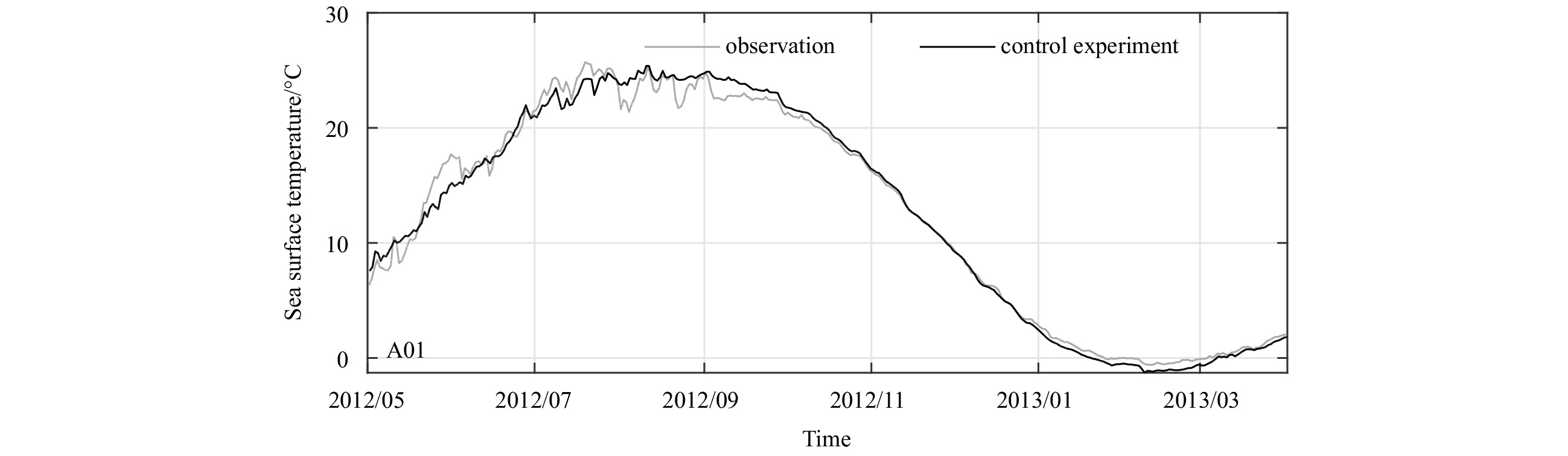
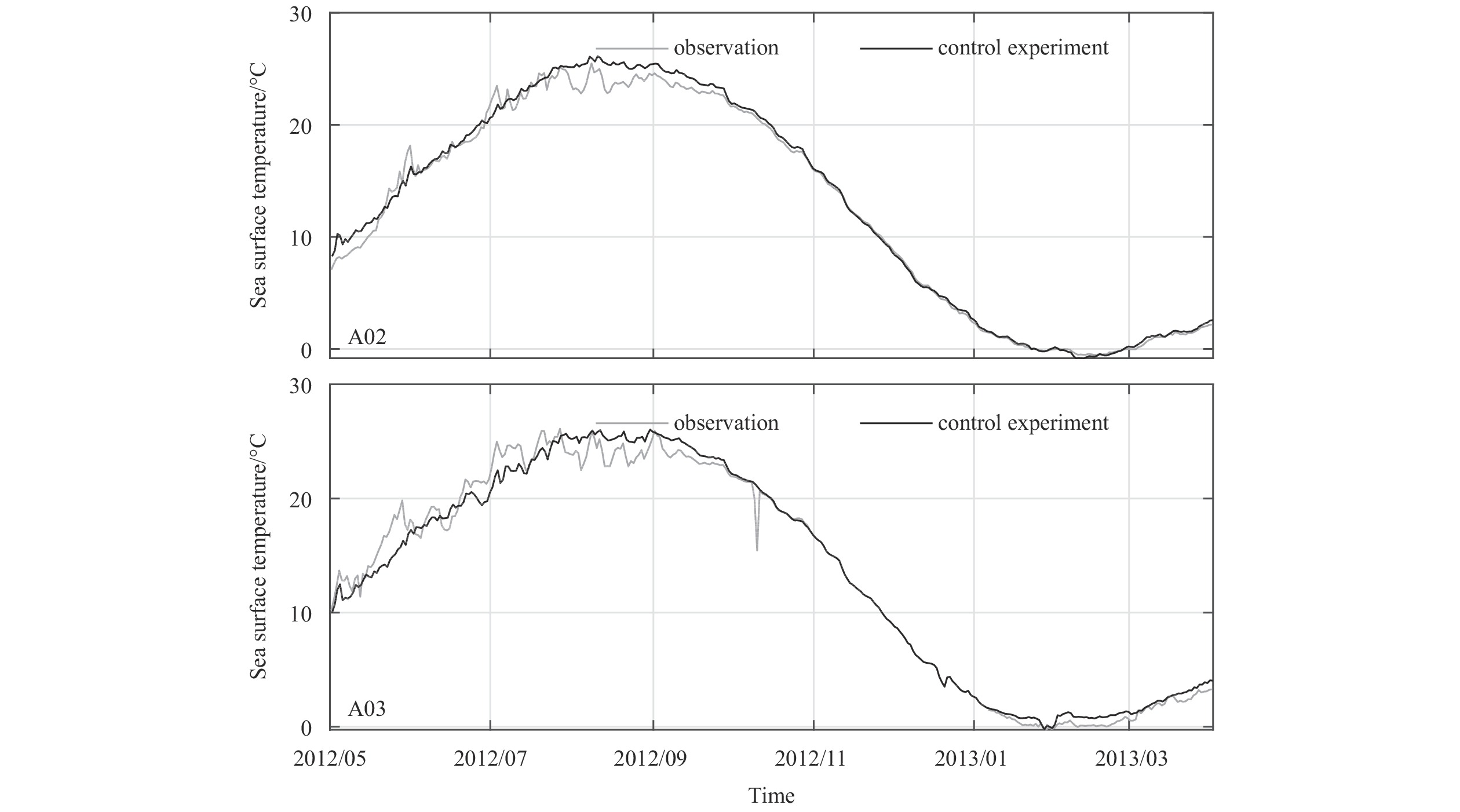
A3. Observed (grey lines) and modelled (black lines) sea surface temperature at three located marked by blue triangles in Fig. 1.
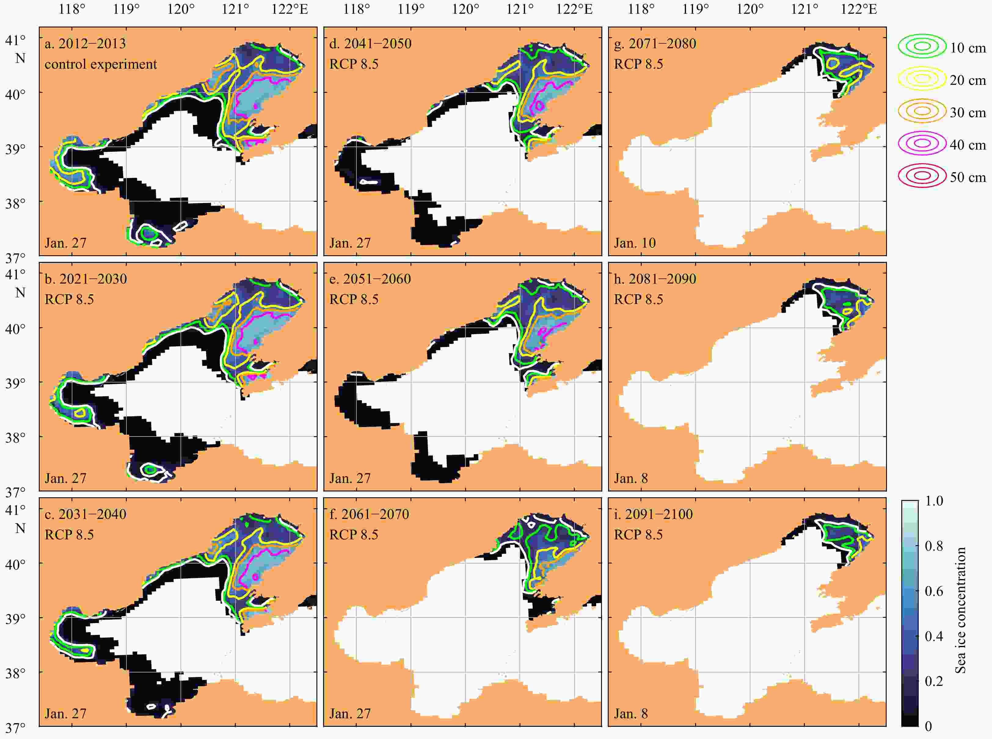
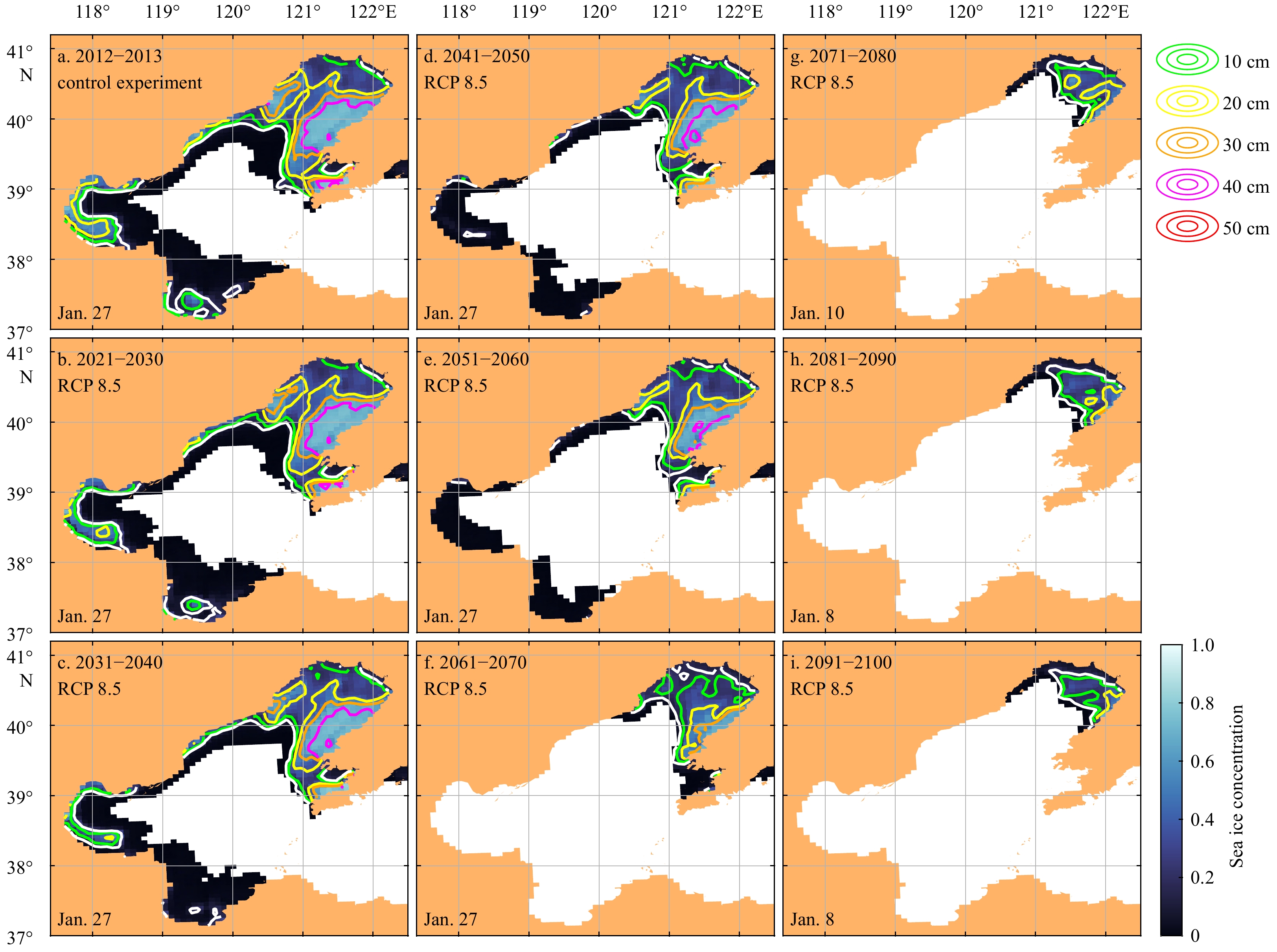
A4. Sea ice concentration (background color) and sea ice thickness (colorful contours) in the control experiment for the winter of 2012–2013 (a) and the sensitive experiments Exp-SE-a for the future in the RCP 8.5 scenario (b–i). The white contours indicate the 15% concentration of sea ice. Only the results with maximum sea ice extent in each experiment are shown.
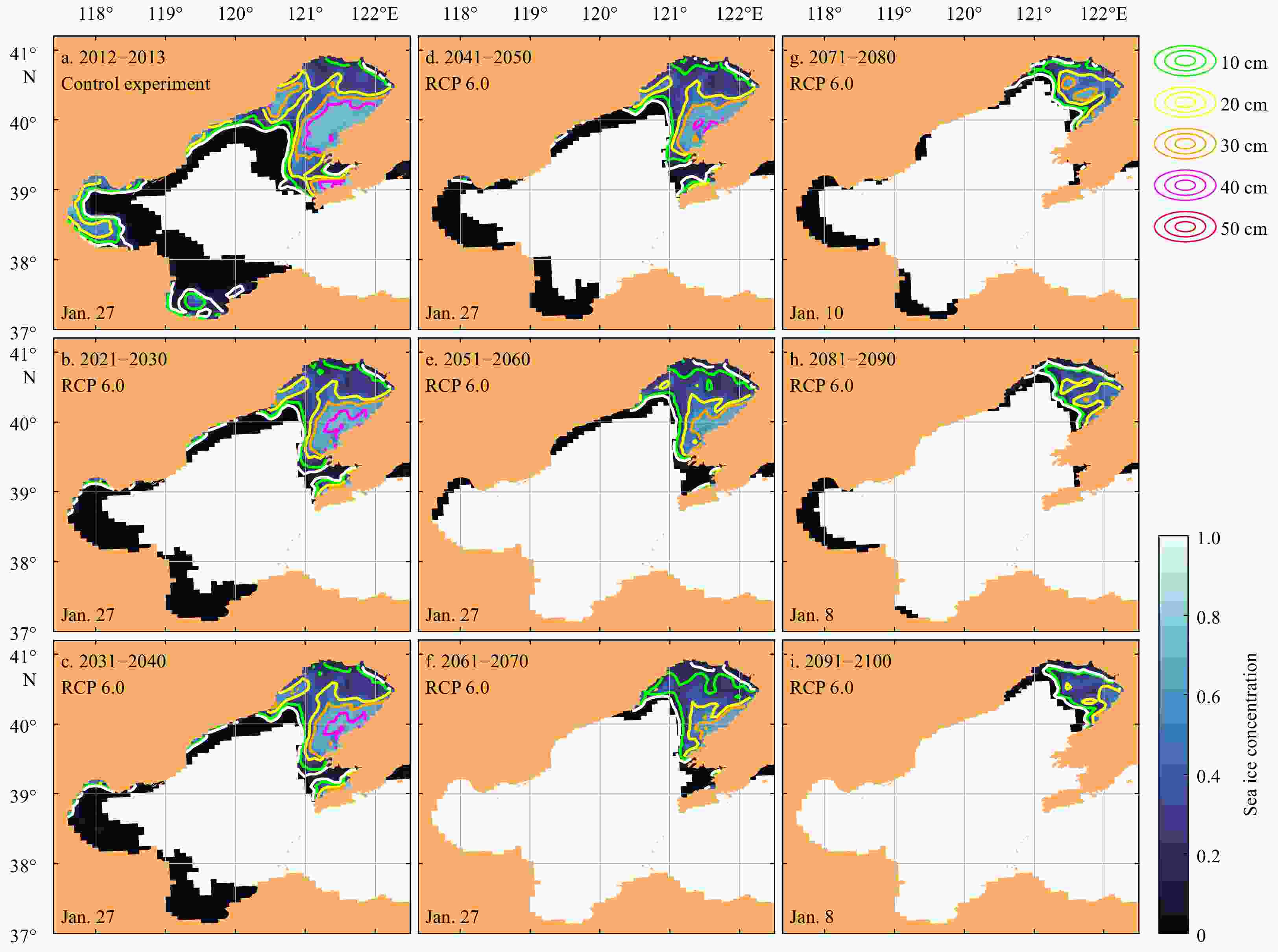
A5. Sea ice concentration (background color) and sea ice thickness (colorful contours) in the control experiment for the winter of 2012–2013 (a) and the sensitive experiments Exp-SE-a for the future in the RCP 6.0 scenario (b–i). The white contours indicate the 15% concentration of sea ice. Only the results with maximum sea ice extent in each experiment are shown.
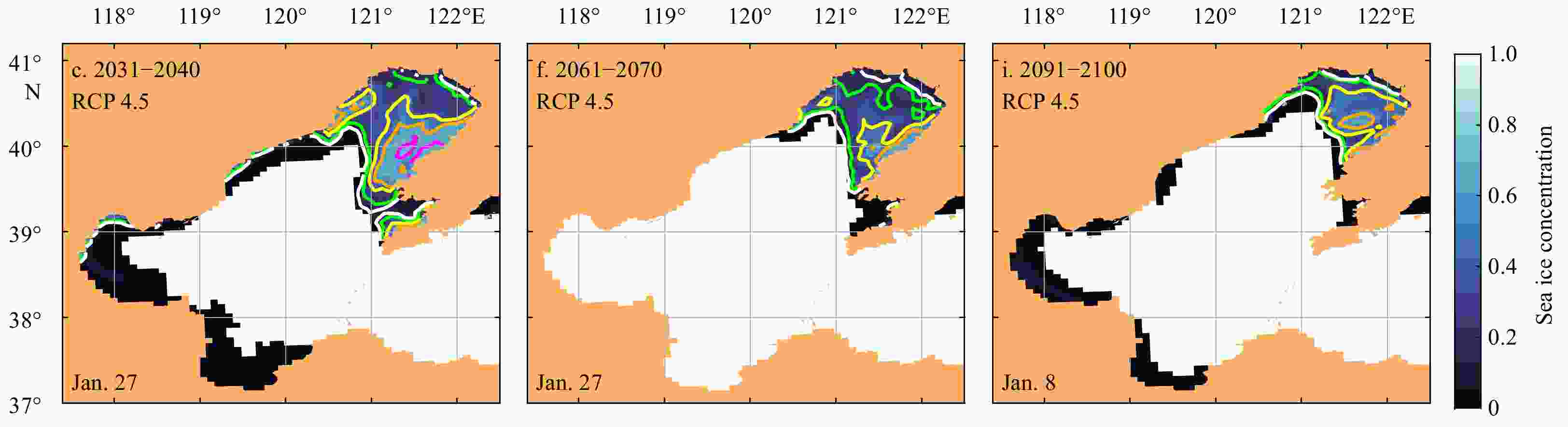
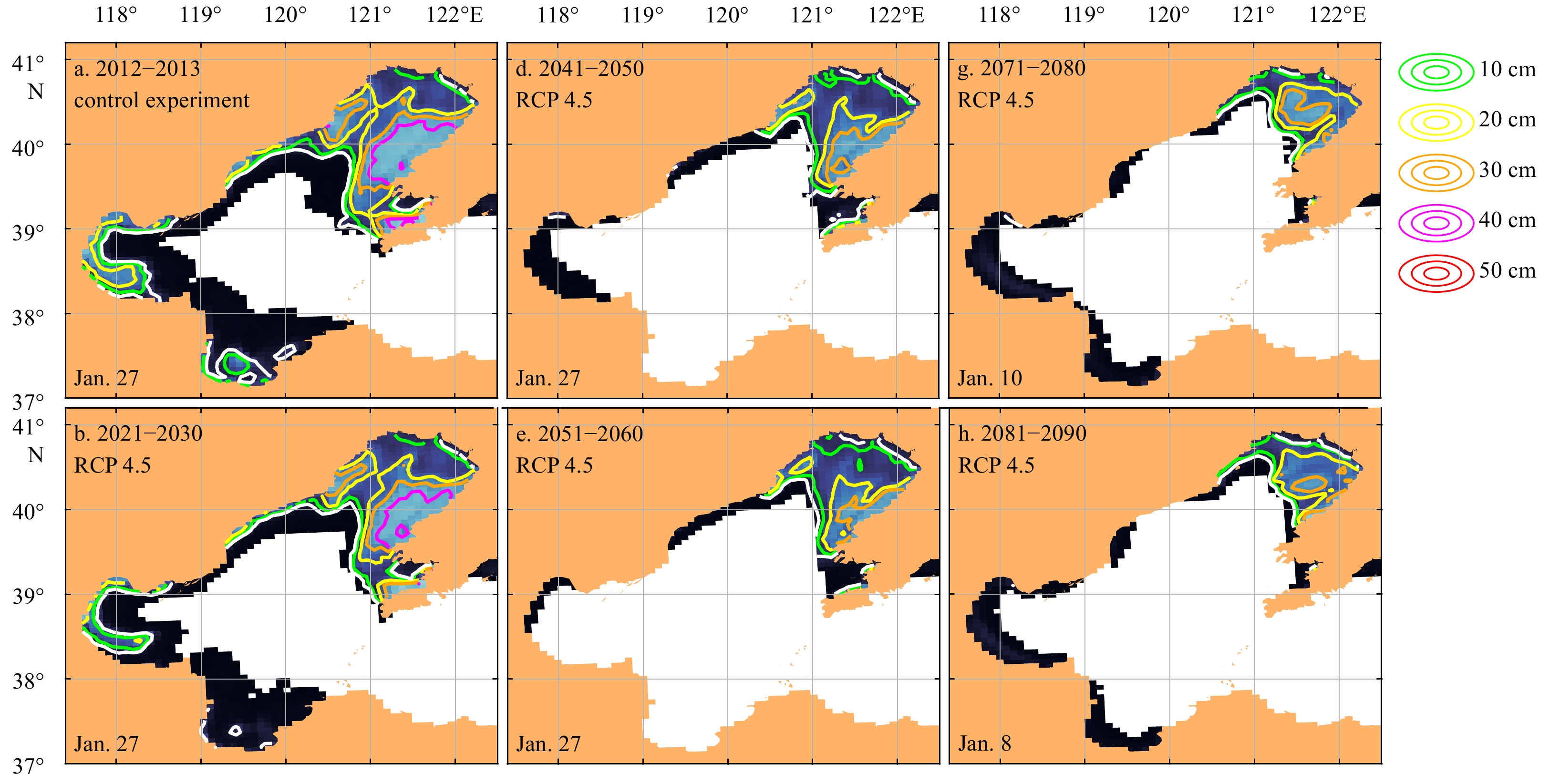
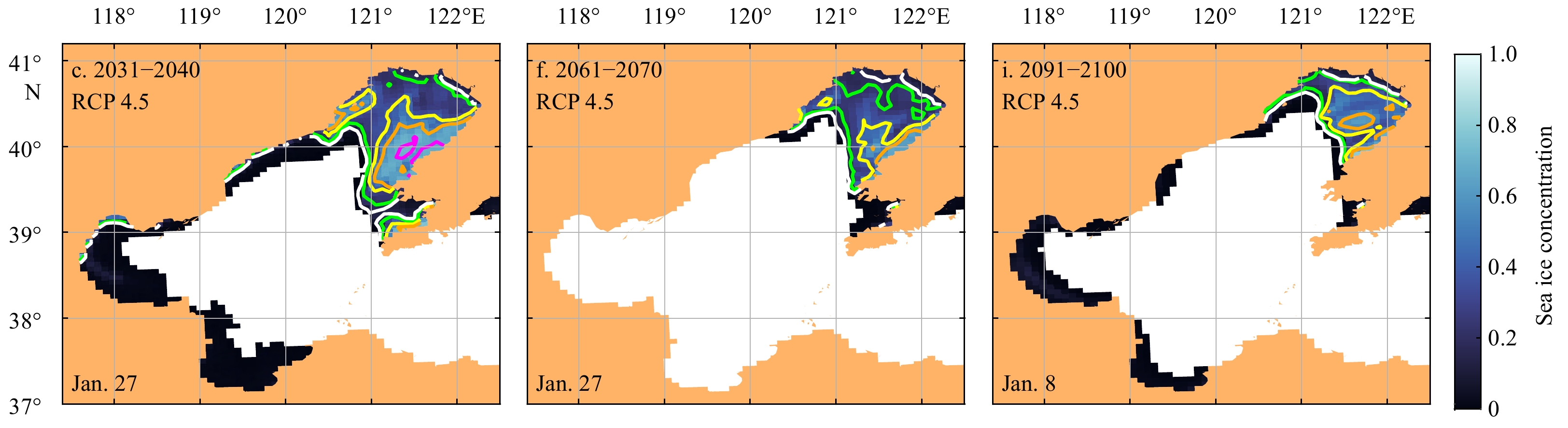
A6. Sea ice concentration (background color) and sea ice thickness (colorful contours) in the control experiment for the winter of 2012–2013 (a) and the sensitive experiments Exp-SE-a for the future in the RCP 4.5 scenario (b–i). The white contours indicate the 15% concentration of sea ice. Only the results with maximum sea ice extent in each experiment are shown.
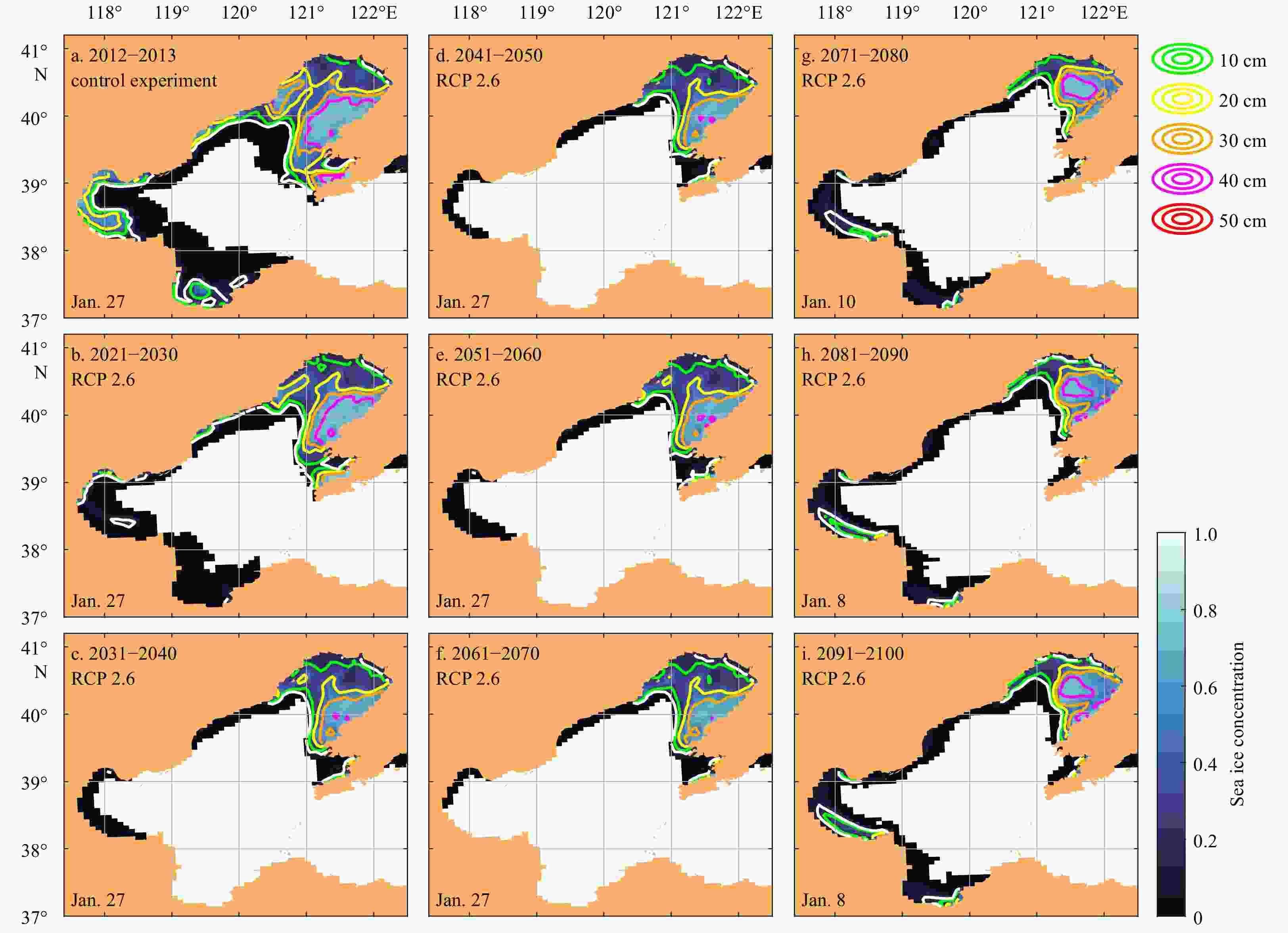
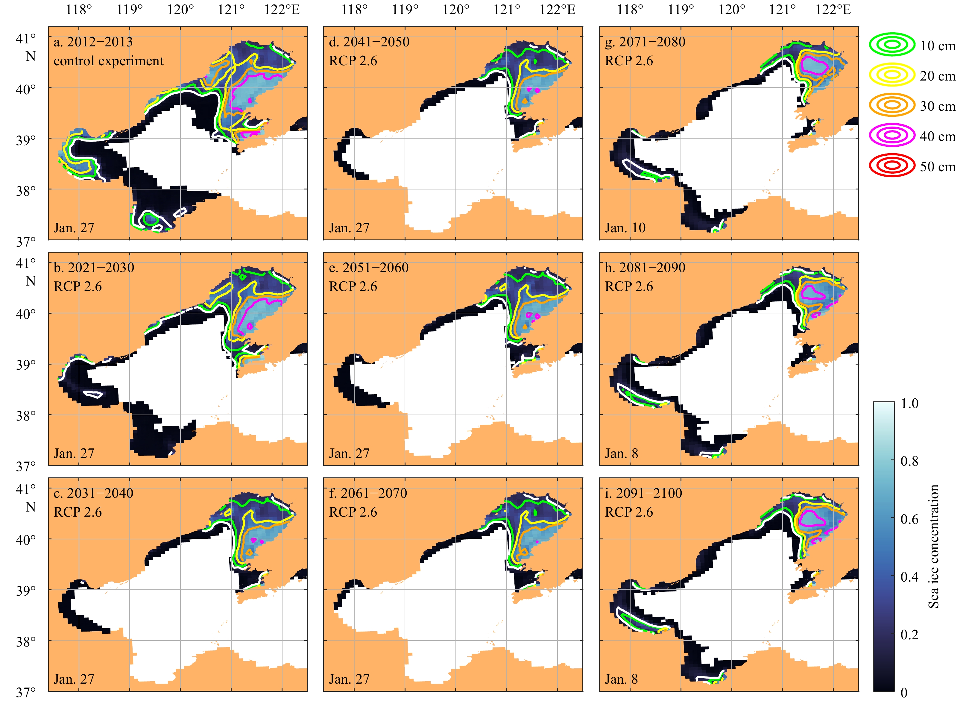
A7. Sea ice concentration (background color) and sea ice thickness (colorful contours) in the control experiment for the winter of 2012–2013 (a) and the sensitive experiments Exp-SE-a for the future in the RCP 2.6 scenario (b–i). The white contours indicate the 15% concentration of sea ice. Only the results with maximum sea ice extent in each experiment are shown.
Table 1. Sources of mean state of atmosphere in different CO2 emission scenarios
Scenario Model Ensemble members Reference RCP 8.5 GFDL-GSM2M r10i1p1–r19i1p1 Rodgers et al. (2015) RCP 6.0 HadGEM2-ES r1i1p1–r4i1p1 Collins et al. (2011) RCP 4.5 CSIRO-MK3.6 r1i1p1–r10i1p1 Rotstayn et al. (2010) RCP 2.6 CanESM2M r1i1p1–r5i1p1 Arora et al. (2011)  下载: 导出CSV
A1. Change in wintertime (November to March) atmospheric conditions in the RCP 8.5 scenario compared to the winter of 2012–2013
Period Specific humidity/
(10–6 kg·kg–1)Precip/
(10–6 kg·m–2·s–1)DLW/
(W·m–2)DSW/
(W·m–2)Air
temperature/°CZonal wind
speed/(m·s−1)Meridional wind
speed/(m·s−1)2021–2030 25.778 –1.168 0.419 0.664 0.366 0.121 0.011 2031–2040 –4.295 –2.028 0.934 2.967 0.744 0.160 0.028 2041–2050 126.452 –1.443 3.601 3.965 1.169 0.221 0.010 2051–2060 196.402 –0.406 6.185 3.297 1.368 0.112 0.002 2061–2070 357.875 0.146 10.523 9.757 2.285 0.147 0.033 2071–2080 568.938 2.331 15.989 25.236 3.349 0.170 0.062 2081–2090 628.251 2.028 17.717 25.554 3.550 0.140 0.016 2091–2100 723.334 2.475 19.798 25.913 4.098 0.151 0.067 Note: DSW and DLW indicate the surface downward shortwave radiation and the surface downward longwave radiation, respectively.
下载: 导出CSV
A2. Change in wintertime (November to March) atmospheric conditions in the RCP 6.0 scenario compared to the winter of 2012–2013
Period Specific humidity/
(10–6 kg·kg–1)Precip/
(10–6 kg·m–2·s–1)DLW/
(W·m–2)DSW
(W·m–2)Air
temperature/°CZonal wind
speed/(m·s–l)Meridional wind
speed/(m·s–l)2021–2030 204.237 –0.615 4.648 –0.407 1.339 0.164 0.277 2031–2040 170.118 –0.646 4.697 –0.736 1.373 0.134 0.301 2041–2050 263.688 –0.378 7.890 –1.925 1.680 0.152 0.245 2051–2060 289.583 –0.893 9.195 0.508 2.628 0.157 0.356 2061–2070 386.868 –0.545 11.638 0.213 2.846 0.163 0.304 2071–2080 548.500 –0.141 15.669 0.965 3.665 0.135 0.292 2081–2090 634.748 0.023 17.757 2.326 4.189 0.185 0.309 2091–2100 740.741 –0.137 19.990 2.700 4.737 0.232 0.385 Note: DSW and DLW indicate the surface downward shortwave radiation and the surface downward longwave radiation, respectively.
下载: 导出CSV
A3. Change in wintertime (November to March) atmospheric conditions in the RCP 4.5 scenario compared to the winter of 2012–2013
Period Specific humidity/
(10–6 kg·kg–1)Precip/
(10–6 kg·m–2·s–1)DLW/
(W·m–2)DSW
(W·m–2)Air
temperature/°CZonal wind
speed/(m·s–l)Meridional wind
speed/(m·s–l)2021–2030 102.536 0.655 2.829 –0.935 0.542 0.033 0.158 2031–2040 234.775 1.504 5.913 0.315 1.020 –0.003 0.221 2041–2050 344.460 1.941 8.611 1.225 1.504 –0.059 0.262 2051–2060 431.652 2.538 10.616 1.740 1.817 –0.045 0.289 2061–2070 539.022 2.861 12.811 2.294 2.227 –0.111 0.304 2071–2080 580.075 2.924 14.104 2.051 2.331 –0.105 0.307 2081–2090 617.175 3.163 14.758 2.141 2.454 –0.087 0.350 2091–2100 613.910 3.163 14.867 2.167 2.488 –0.098 0.329 Note: DSW and DLW indicate the surface downward shortwave radiation and the surface downward longwave radiation, respectively.
下载: 导出CSV
A4. Change in wintertime (November to March) atmospheric conditions in the RCP 2.6 scenario compared to the winter of 2012–2013
Period Specific humidity/
(10–6 kg·kg–1)Precip/
(10–6 kg·m–2·s–1)DLW/
(W·m–2)DSW
(W·m–2)Air
temperature/°CZonal wind
speed/(m·s–l)Meridional wind
speed/(m·s–l)2021–2030 169.520 0.049 –0.221 6.450 0.729 0.379 0.189 2031–2040 395.981 0.077 3.033 8.581 1.517 0.381 0.420 2041–2050 385.460 –0.017 2.982 10.611 1.488 0.416 0.329 2051–2060 350.707 –0.013 2.875 10.532 1.276 0.333 0.308 2061–2070 387.610 –1.115 2.174 12.442 1.564 0.358 0.332 2071–2080 399.049 –1.762 2.424 12.674 1.526 0.385 0.352 2081–2090 350.722 –1.659 1.158 13.290 1.395 0.559 0.314 2091–2100 300.425 –1.071 –0.015 13.855 1.098 0.510 0.327 Note: DSW and DLW indicate the surface downward shortwave radiation and the surface downward longwave radiation, respectively.
下载: 导出CSV
-
[1] Amante C, Eakins B W. 2009. ETOPO1 1 arc-minute global relief model: procedures, data sources and analysis. NOAA Technical Memorandum NESDIS NGDC-24. Bouder, Colorado, USA: National Centers for Environmental Information, NOAA, https://www.ncei.noaa.gov/access/metadata/landing-page/bin/iso?id=gov.noaa.ngdc.mgg.dem:316 [2] Arora V K, Scinocca J F, Boer G J, et al. 2011. Carbon emission limits required to satisfy future representative concentration pathways of greenhouse gases. Geophysical Research Letters, 38(5): L05805. doi: 10.1029/2010GL046270 [3] Bian Changwei, Jiang Wensheng, Pohlmann T, et al. 2016. Hydrography-physical description of the Bohai Sea. Journal of Coastal Research, 74(10074): 1–12. doi: 10.2112/SI74-001.1 [4] Chen Changsheng, Liu Hedong, Beardsley R C. 2003. An unstructured grid, finite-volume, three-dimensional, primitive equations ocean model: application to coastal ocean and estuaries. Journal of Atmospheric and Oceanic Technology, 20(1): 159–186. doi: 10.1175/1520-0426(2003)020<0159:AUGFVT>2.0.CO;2 [5] Collins W J, Bellouin N, Doutriaux-Boucher M, et al. 2011. Development and evaluation of an Earth-System model–HadGEM2. Geoscientific Model Development, 4(4): 1051–1075. doi: 10.5194/gmd-4-1051-2011 [6] Dai Aiguo, Qian Taotao, Trenberth K E, et al. 2009. Changes in continental freshwater discharge from 1948 to 2004. Journal of Climate, 22(10): 2773–2792. doi: 10.1175/2008JCLI2592.1 [7] Egbert G D, Erofeeva S Y. 2002. Efficient inverse modeling of barotropic ocean tides. Journal of Atmospheric and Oceanic Technology, 19(2): 183–204. doi: 10.1175/1520-0426(2002)019<0183:EIMOBO>2.0.CO;2 [8] Fichefet T, Maqueda M A M. 1997. Sensitivity of a global sea ice model to the treatment of ice thermodynamics and dynamics. Journal of Geophysical Research: Oceans, 102(C6): 12609–12646. doi: 10.1029/97JC00480 [9] Flather R A. 1994. A storm surge prediction model for the northern bay of Bengal with application to the cyclone disaster in April 1991. Journal of Physical Oceanography, 24(1): 172–190. doi: 10.1175/1520-0485(1994)024<0172:ASSPMF>2.0.CO;2 [10] Goosse H, Fichefet T. 1999. Importance of ice-ocean interactions for the global ocean circulation: a model study. Journal of Geophysical Research: Oceans, 104(C10): 23337–23355. doi: 10.1029/1999JC900215 [11] Ji Qiyan, Zhu Xueming, Wang Hui, et al. 2015. Assimilating operational SST and sea ice analysis data into an operational circulation model for the coastal seas of China. Acta Oceanologica Sinica, 34(7): 54–64. doi: 10.1007/s13131-015-0691-y [12] Karvonen J, Shi Lijian, Cheng Bin, et al. 2017. Bohai sea ice parameter estimation based on thermodynamic ice model and earth observation data. Remote Sensing, 9(3): 234. doi: 10.3390/rs9030234 [13] Large W G, Yeager S G. 2004. Diurnal to Decadal Global Forcing for Ocean and Sea-Ice Models: The Data Sets and Flux Climatologies. NCAR/TN-460+STR. Boulder, Colorado: National Center for Atmospheric Research, doi: 10.5065/D6KK98Q6, https://opensky.ucar.edu/islandora/object/technotes:434 [14] Madec G, Imbard M. 1996. A global ocean mesh to overcome the North Pole singularity. Climate Dynamics, 12(6): 381–388. doi: 10.1007/BF00211684 [15] Madec G, Bourdallé-Badie R, Bouttier P A, et al. 2008. NEMO ocean engine. Zenodo: Notes du Pôle de modélisation de l'Institut Pierre-Simon Laplace (IPSL), https://doi.org/10.5281/zenodo.3248739 [16] Ning Li, Xie Feng, Gu Wei, et al. 2009. Using remote sensing to estimate sea ice thickness in the Bohai Sea, China based on ice type. International Journal of Remote Sensing, 30(17): 4539–4552. doi: 10.1080/01431160802592542 [17] Ouyang Lunxi, Hui Fengming, Zhu Lixian, et al. 2019. The spatiotemporal patterns of sea ice in the Bohai Sea during the winter seasons of 2000–2016. International Journal of Digital Earth, 12(8): 893–909. doi: 10.1080/17538947.2017.1365957 [18] Rodgers K B, Lin J, Frölicher T L. 2015. Emergence of multiple ocean ecosystem drivers in a large ensemble suite with an Earth system model. Biogeosciences, 12(11): 3301–3320. doi: 10.5194/bg-12-3301-2015 [19] Rotstayn L D, Collier M A, Dix M R, et al. 2010. Improved simulation of Australian climate and ENSO-related rainfall variability in a global climate model with an interactive aerosol treatment. International Journal of Climatology, 30(7): 1067–1088. doi: 10.1002/joc.1952 [20] Saha S, Moorthi S, Wu Xingren, et al. 2014. The NCEP climate forecast system version 2. Journal of Climate, 27(6): 2185–2208. doi: 10.1175/JCLI-D-12-00823.1 [21] Shi Wei, Wang Menghua. 2012a. Sea ice properties in the Bohai Sea measured by MODIS-Aqua: 1. Satellite algorithm development. Journal of Marine Systems, 95: 32–40. doi: 10.1016/j.jmarsys.2012.01.012 [22] Shi Wei, Wang Menghua. 2012b. Sea ice properties in the Bohai Sea measured by MODIS-Aqua: 2. Study of sea ice seasonal and interannual variability. Journal of Marine Systems, 95: 41–49. doi: 10.1016/j.jmarsys.2012.01.010 [23] Su Hua, Ji Bowen, Wang Yunpeng. 2019. Sea ice extent detection in the Bohai Sea using sentinel-3 OLCI data. Remote Sensing, 11(20): 2436. doi: 10.3390/rs11202436 [24] Su Hua, Wang Yunpeng. 2012. Using MODIS data to estimate sea ice thickness in the Bohai Sea (China) in the 2009–2010 winter. Journal of Geophysical Research: Oceans, 117(C10): C10018. doi: 10.1029/2012JC008251 [25] Su Hua, Wang Yunpeng, Yang Jingxue. 2012. Monitoring the spatiotemporal evolution of sea ice in the Bohai Sea in the 2009-2010 winter combining MODIS and meteorological data. Estuaries and Coasts, 35(1): 281–291. doi: 10.1007/s12237-011-9425-3 [26] Umlauf L, Burchard H. 2003. A generic length-scale equation for geophysical turbulence models. Journal of Marine Research, 61(2): 235–265. doi: 10.1357/002224003322005087 [27] Umlauf L, Burchard H. 2005. Second-order turbulence closure models for geophysical boundary layers. A review of recent work. Continental Shelf Research, 25(7–8): 795–827. doi: 10.1016/j.csr.2004.08.004 [28] van Vuuren D P, Edmonds J, Kainuma M, et al. 2011. The representative concentration pathways: an overview. Climatic Change, 109: 5. doi: 10.1007/s10584-011-0148-z [29] Yan Yu, Gu Wei, Xu Yingjun, et al. 2019. The in situ observation of modelled sea ice drift characteristics in the Bohai Sea. Acta Oceanologica Sinica, 38(3): 17–25. doi: 10.1007/s13131-019-1395-5 [30] Yan Yu, Shao Dongdong, Gu Wei, et al. 2017. Multidecadal anomalies of Bohai Sea ice cover and potential climate driving factors during 1988–2015. Environmental Research Letters, 12(9): 094014. doi: 10.1088/1748-9326/aa8116 [31] Yan Yu, Uotila P, Huang Kaiyue, et al. 2020. Variability of sea ice area in the Bohai Sea from 1958 to 2015. Science of the Total Environment, 709: 136164. doi: 10.1016/j.scitotenv.2019.136164 [32] Yuan Shuai, Gu Wei, Xu Yingjun, et al. 2012. The estimate of sea ice resources quantity in the Bohai Sea based on NOAA/AVHRR data. Acta Oceanologica Sinica, 31(1): 33–40. doi: 10.1007/s13131-012-0173-4 [33] Yuan Shuai, Liu Chengyu, Liu Xueqin. 2018. Practical model of sea ice thickness of Bohai Sea based on MODIS data. Chinese Geographical Science, 28(5): 863–872. doi: 10.1007/s11769-018-0986-y [34] Zhang Na, Wang Jin, Wu Yongsheng, et al. 2019. A modelling study of ice effect on tidal damping in the Bohai Sea. Ocean Engineering, 173: 748–760. doi: 10.1016/j.oceaneng.2019.01.049 [35] Zhang Na, Wu Yongsheng, Zhang Qinghe. 2015. Detection of sea ice in sediment laden water using MODIS in the Bohai Sea: a CART decision tree method. International Journal of Remote Sensing, 36(6): 1661–1674. doi: 10.1080/01431161.2015.1015658 [36] Zu Ziqing, Ling Tiejun, Zhang Yunfei, et al. 2016. Future projection of the sea ice in the Bohai Sea and the North Yellow Sea. Marine Forecasts (in Chinese), 33(5): 1–8 -


 点击查看大图
计量
- 文章访问数: 657
- HTML全文浏览量: 194
- PDF下载量: 14
- 被引次数: 0

